This is a follow-up to the part I post about using WSJT-X modes through a linear transponder on a LEO satellite. In part I, we considered the tolerance of several WSJT-X modes to the residual Doppler produced by a temporal offset in the Doppler computation used for computer Doppler correction. There, we introduced a parameter  which represents the time shift between the real Doppler curve and the computed Doppler curve. The main idea was that a decoder could try to correct the residual Doppler by trying several values of until a decode is produced.
Here we examine the effect of TLE age on the accuracy of the Doppler computation. The problem is that, when a satellite pass occurs, TLEs have been calculated at an epoch in the past, so there is an error between the actual Doppler curve and the Doppler curve predicted by the TLEs. We show that the actual Doppler curve is very well approximated by applying a time shift to the Doppler curve predicted by the TLEs, justifying the study in part I.
We look at the same pass that we studied in part I: the 2017/7/9 03:12:00 UTC pass of LilacSat-1 over my station (40.6007, -3.7080, 700m ASL). The TLE in Space-Track whose epoch is nearest to the time of the pass is
1 42725U 98067ME  17189.87025697 +.00007644 +00000-0 +11689-3 0  9999
2 42725 051.6407 289.9183 0007265 030.1333 330.0075 15.55443398006852
Note that this TLE is different from the one used in part I. Presumably, this TLE wasn't available yet when I started writing part I. We will assume that this TLE predicts the actual Doppler curve. Actually, this TLE was measured 6 hours and 23 minutes before the pass.
Typically, we don't have access to such a current TLE during the time of the pass, so we have to do our Doppler prediction using an older TLE. For instance, when I started writing part I, the TLE I used was the most current and it had an epoch of 2017/07/07 19:45:24. The pass I selected was the next overhead pass over my station.
Now let us look at the problem of predicting the Doppler with an older TLE. To exaggerate the effects, I have selected the TLE
1 42725U 98067ME  17183.50952476 +.00011042 +00000-0 +16628-3 0  9992
2 42725 051.6406 321.6862 0006959 008.0741 352.0361 15.55338480005862
which was measured 6 days and 9 hours before the TLE I am taking as current. The figure below shows the different downlink Doppler curves. The downlink frequency is taken as 436.5MHz, in the middle of the 70cm Amateur satellite band.
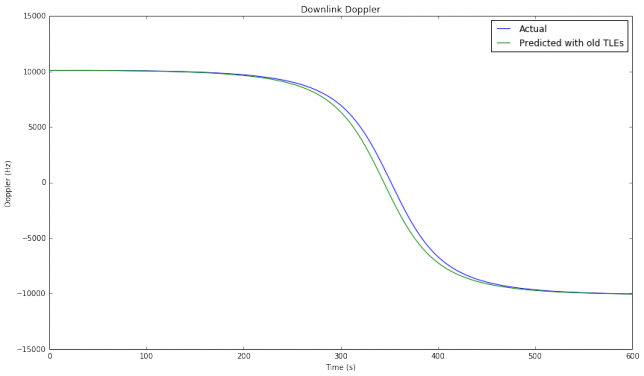
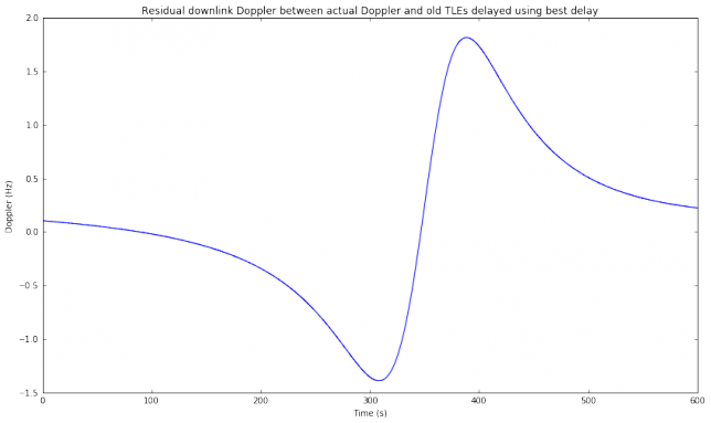
We can see that the actual Doppler curve looks very much like a time shifted version of the predicted Doppler curve. Therefore, applying an adequate time shift to the predicted curve yields a very good approximation of the actual Doppler. A simple way to compute this is as the difference between the times where each Doppler curve is zero (which correspond to the times of closes approach). This difference, called "best delay", is 7.38 seconds in this case. In the figure below we see that the difference between the actual Doppler and the predicted Doppler shifted by 7.38 seconds is only of a few Hz.
A decoder trying to correct the residual Doppler will test different values of until a decode is produced. The thresholds obtained in part I show how precise the search for the correct needs to be depending on the mode.
To study the effect of TLE age in the Doppler prediction, we compute the best delay for all the TLEs in Space-Track taken during the week before the pass. The results are shown in the figures below. The second figure is just a zoomed-in portion of the first figure.

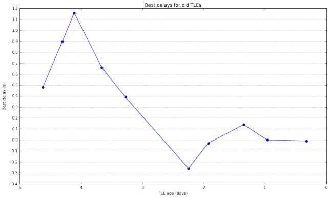
These figures are very interesting. The difference in best delay between two consecutive points is a measure of how much the TLE parameters are changing because the orbit of the satellite deviates from the prediction done by the SGP model. We see that sometimes the satellite deviates much from the SGP model, causing changes of several seconds in the best delay, while other times the changes in the best delay are small. These effects should be studied for several satellites over longer time spans. Perhaps I'll do it in a future post.
The conclusion of these figures is that sometimes the best delay can be on the order of several seconds, perhaps as high as 10 seconds. However, many times, if using the latest TLEs available, the best delay will be on the order of a few hundreds of ms. This means that it is possible for a decoder to try in real time different values of until a decode is found. For instance, if using FT8, a step of 0.25 seconds in the search for can be used.
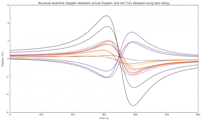
The figure below shows the residual downlink Doppler when correcting each of the old TLEs with the best delay computed above. The age of the TLEs is encoded using the inferno colormap, with older TLEs in black and newer TLEs in yellow. We see that the residual Doppler is very small in all cases. This means that most of the error produced by using older TLEs happens in the along-orbit component of the position of the satellite.
So far we have only concerned ourselves with the downlink Doppler. A strategy to deal with the residual downlink Doppler is now clear: try different values of until most of the residual Doppler is compensated and a decode is obtained. This still leaves us the question of what to do with the uplink Doppler, since a search for the correct Doppler cannot be conducted while transmitting. Here there are some useful ideas.
First, the transmitting station can estimate the best delay parameter by listening to their own transmissions. The self-Doppler (the Doppler with which the transmitting station hears their own transmissions) is always proportional to the downlink Doppler for the transmitting station. Indeed, it is the same as a downlink Doppler for a signal whose frequency is the difference between the downlink frequency and the uplink frequency, or the sum of the downlink and uplink frequencies, according as to whether the linear transponder is inverting (the usual case) or non-inverting. Therefore, the transmitting station can search for by trying to decode their own transmissions. When a good is found, this value of can be used by the transmitting station to correct the residual uplink Doppler in its transmission. Note that this only compensates the residual uplink Doppler up to some extent, since the value of is obtained just by searching for a correct decode and some modes have a rather high threshold for , as we have seen in part I. Still, this correction can be enough, especially if the uplink is at a lower frequency than the downlink.
The same best delay parameter can be used by stations anywhere in the world and remains valid for a time interval of at least several hours. Therefore, it can be regarded as a correction to the published TLEs and shared over the internet or even in WSJT-X messages through the satellite transponder. Also, some stations can carry out a more precise calculation of the best delay rather than listening to their own transmissions, which are supposed to be weak. The precise downlink Doppler can be analysed by listening to the satellite beacon, when it is available, or by transmitting a strong carrier through the transponder and measuring the self-Doppler.
Residual uplink Doppler correction can also be carried out by a search in the receiving station, similarly to how downlink Doppler is corrected. However, this requires that the receiving station knows the location of the transmitting station and adds another search parameter, so it is not a feasible option in general.
Finally, there are some things that can help, even if no measures to correct for residual uplink Doppler are taken. If the satellite is mode V/U (uplink on 145MHz and downlink on 435MHz), then the uplink Doppler is around one third of the downlink Doppler, so the correction for the uplink is not so critical. Unfortunately, most of the linear transponders these days are mode U/V (uplink on 435MHz and downlink on 145MHz), which is a more difficult situation. We have also noted that the situation with residual Doppler is only difficult near the closest approach of an overhead pass. At other times in the pass and also for non-overhead passes, the rate of change in Doppler is not so large. At any given time, the number of stations that have the satellite directly overhead represents a small proportion of all the stations that have the satellite in view, so we can expect that most of the transmissions do not have to cope with such a large rate of change in Doppler.
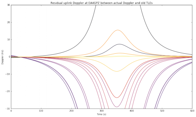
As an example of these ideas, the figure below shows the residual uplink Doppler at my station when the old TLEs are not compensated ( ). You can get an idea of which residual Doppler curves can still be handled by the WSJT-X decoder by looking at the figures in part I. We see that only the newest TLEs have an acceptable residual Doppler when no compensation is done with . Here it helps the fact that the uplink frequency is taken as 145.9MHz, in the middle of the 2m Amateur satellite band, as would be the case for a V/U transponder.
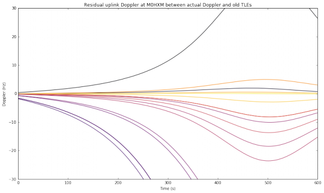
However, if we now look at a transmitting station in other location, things can change. We now look to the location of M0HXM, in Newcastle upon Tyne, as a transmitting station. This is not an overhead pass for M0HXM, so the residual Doppler is smaller and most old TLEs can be used without compensation.
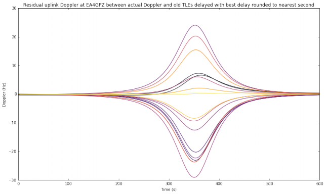
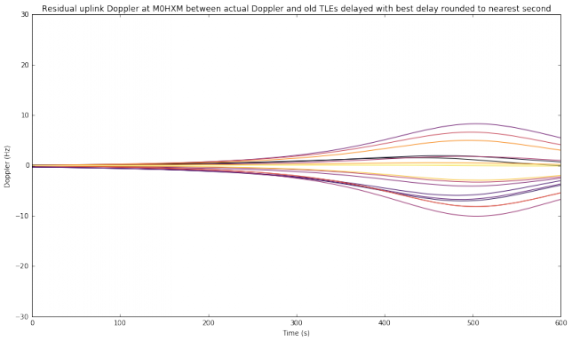
Now we assume that the transmitting station is able to approximate the best delay to the nearest second by using any of the methods outlined above. Note that approximating to the nearest second is a rather coarse approximation. It is likely that better precision can be obtained just by listening to your own transmissions. The situation now is quite good: all the transmissions by EA4GPZ and M0HXM have an acceptable residual uplink Doppler, even when the oldest TLEs are used.
In conclusion, using the techniques described in this post and part I, WSJT-X modes such as FT8 and QRA64E can be usable under all circumstances with a V/U linear transponder, and probably under many circumstances with a U/V linear transponder. Now it is just a matter of running some on-air tests to validate the techniques. Recently, there have been some people successfully using FT8 through some LEO satellites, but only for low elevations, where the rate of change of Doppler is small. As far as I know, the case of high elevations is still untested, as it requires special residual Doppler correction techniques such as those described here.
The computations used in this post have been done in this Jupyter notebook.