This weekend I have recorded the full EAPSK63 Spanish PSK63 contest in the 40m band with the goal of playing back the recording later and reporting the stations showing excessively high IMD levels. In PSK contests, it is usual to see terribly distorted signals, which are the result of reckless operating techniques and stations which are setup inadequately. Contest rules don't help much, as they are usually too weak to prevent distorted signals from interfering other participants. Amateurs should take care and strive to produce a signal as clean as possible. For instance, in the US, Part 97 101 a) states that "each amateur station must be operated in accordance with good engineering and good amateur practice". Here I describe the signal processing done in this study and list a "hall of shame" of the worst stations I have spotted in my recording. I will notify by email the contest manager and all the stations in this list with the hope that the situation improves in the future.

Some words about IMD

Before passing to the setup of this experiment, let us discuss a few generalities about IMD in Amateur narrowband digital modes such as PSK. A brief introduction to IMD in Amateur PSK modes can be found here. Any signal which doesn't have a constant amplitude will present intermodulation products because the signal processing stages (for instance, the power amplifier) are not perfectly linear. Intermodulation products broaden the bandwidth of the signal, producing interference to adjacent stations.

In a well designed system, these intermodulation products are pretty weak in comparison with the main signal, so the interference they can produce is very limited. For instance, a clean PSK63 signal will fit in a bandwidth of 80 or 100Hz, and everything outside this bandwidth will be very weak. However, a very distorted PSK63 signal can occupy more than 600Hz, potentially causing interference to many stations. IMD (or intermodulation distortion) is just a measure of the strength of these undesired intermodulation products, in comparison with the main signal.

Some signals, such as FSK, have a constant amplitude, so they are not distorted when passing through a non-linear stage, and IMD is not a problem. However, for PSK and many other modes, one has to be very careful about non-linearities and IMD.

There are two main causes of excessively high IMD in Amateur digital modes. The first is saturation in the audio chain or the transmitter driven into ALC mode. These problems are very easy to solve with a proper station setup, so there is no reason why this should be the cause of high IMD, yet it seems that this is cause of the problem for many stations.

If the digital signal is fed into the transmitter using an audio signal and a soundcard, the output level of the soundcard shouldn't be too high so that the signal saturates. Of course, clipping should be avoided, but some soundcards get nonlinear for signals near 100% output, so one should also watch out for that and reduce the output level in case this happens. The audio signal fed to the transmitter should be of an adequate level so that the transmitter doesn't saturate either. Usually this is accomplished by means of a resistive voltage divider and/or an option of the transmitter to set audio input gain.

ALC in the transmitter should be disabled or the signal level should be low enough so that the ALC doesn't engage. The proper setup will vary between different transmitter models, but one should know how to set up his computer and transmitter properly. The goal is that a clean RF signal is delivered to the power amplifier. With a proper setup this is always possible.

The second cause is poor performance in the power amplifier. This is a problem because it is not easy to design a class AB push-pull PA which has very good IMD performance when driven near its maximum output power. The easy solution to excessive IMD produced in the amplifier is to reduce output power. Recall that if we reduce the power by 1dB, the IMD products of order will be reduced by dB (and here is an odd number greater or equal than 3), so just reducing the power just a little bit will reduce higher order IMD products by a considerable amount.

The only other solution is to modify the amplifier to improve its performance, perhaps by changing the bias or by using better devices. This is not so easy to do and probably not possible for many Amateurs. However, one should be careful when choosing an amplifier. Some of the cheapest models are badly designed and they should be operated at a significant fraction of their rated maximum power to avoid excessively high IMD. For instance, these tests by Charles W8JI on the RM HLA-150 300W amplifier show that this amplifier should be operated below 90W output power for an acceptable IMD. The amplifiers inside commercial transceivers made by the well-known brands usually perform OK, but still one should be careful not to drive the amplifier near saturation.

About the contest rules in EAPSK63

The only mention of distortion in the rules of the EAPSK63 contest is as follows:

Power: Recommended power maximum 50w, in order not to cause interference or splatter to other participants.

However, as I've described above, higher power is not the main cause of high levels of IMD. The main cause is improper operation and station setup: operators that don't know how to setup their audio and RF signal levels or don't care to do so and operators that don't monitor their transmit signal to check that it's clean.

The worse part about this rule is that it's just a recommendation. Putting something not mandatory in the rules is like not putting anything. Some people will just do anything they can trying to achieve more contacts. They won't follow recommendations. They will only follow rules that are mandatory and enforced with loss of points or disqualifications.

Recording setup

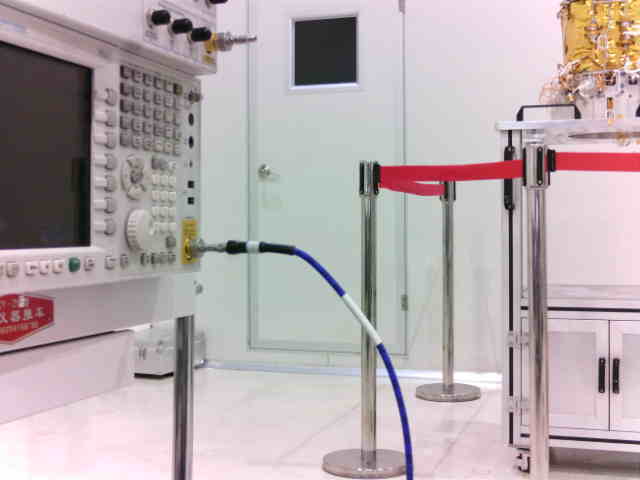
The recording station in this experiment has been my Hermes-Lite 2.0 beta2 board. This is a DDC SDR using the AD9866 12bit frontend at 76.8MHz. The FPGA in this transceiver filters and downsamples the data from the ADC to produce a 24bit 48kHz IQ slice centred at 7.055MHz and streams it over Gigabit Ethernet into my laptop. There, I use gr-hermeslite2 to receive the samples in GNU Radio. The data is saved in a 16bit 48kHz IQ wav file for later processing and also sent into Linrad using gr-linrad for monitoring.

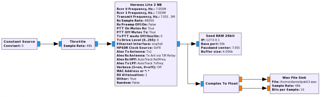
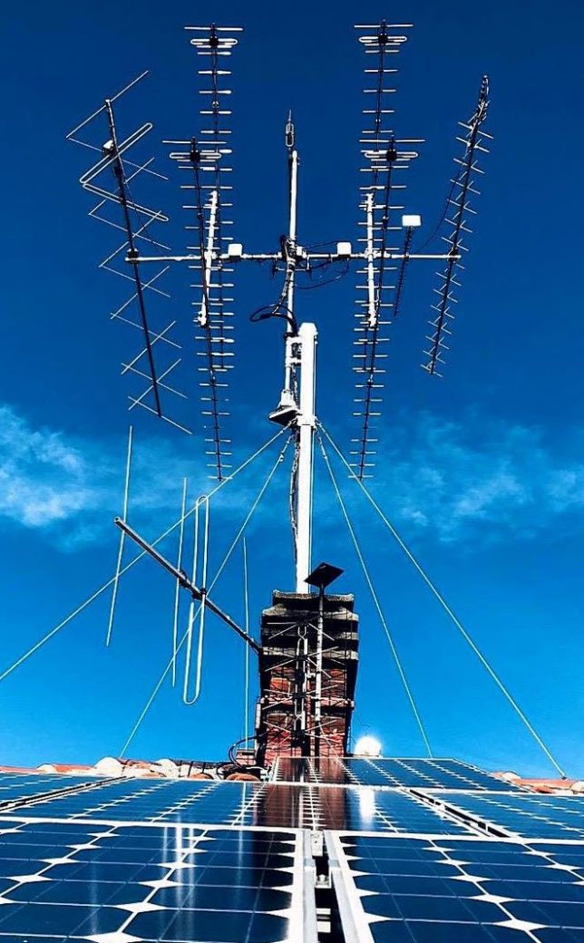
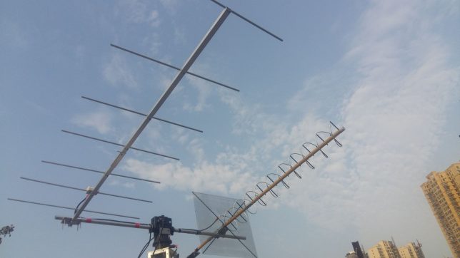
The antenna is a half-wave inverted V dipole for 40m in a not so good location: its feed point is around 8m over the ground, while the tips are almost at ground level. It is also partially occluded by nearby buildings. It is connected to the RX input of the Hermes-Lite 2.0 beta2 without any additional filtering. A gain of 18dB is used in the AD9866. In my RF environment, this setting produces clipping in the ADC only very infrequently.

After the recording finished, about 15 minutes after the end of the contest, stat gives a modification timestamp of 2017-03-12 17:15:11.662109024 +0100. Linrad says that the length of the wav file is 24:30:50. Therefore, we calculate that the start of the recording was 2017-03-11 15:44:21 UTC. The system is running ntpd so this calculation should be accurate to one second. Better resolution can be obtained by counting precisely the number of samples in the wav file, but accuracy of the computer clock is probably not better than 100ms, even with NTP, and one should take into account the delay from the RF input to the computer. The sample rate of the wav file is derived from the TCXO of the Hermes-Lite, which is 0.5ppm. Over a period of 24 hours, this represents an accuracy of 24ms.

I have uploaded the complete wav recording in case anyone wants to do some experiments. The file is pretty large (16GB), so I don't promise to host it forever, but I'll try to leave it as long as possible. The file is eapsk63-7055kHz-2017-03-11-154421.wav

Playback setup

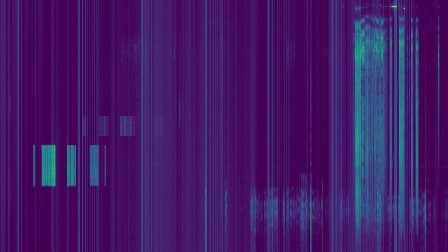
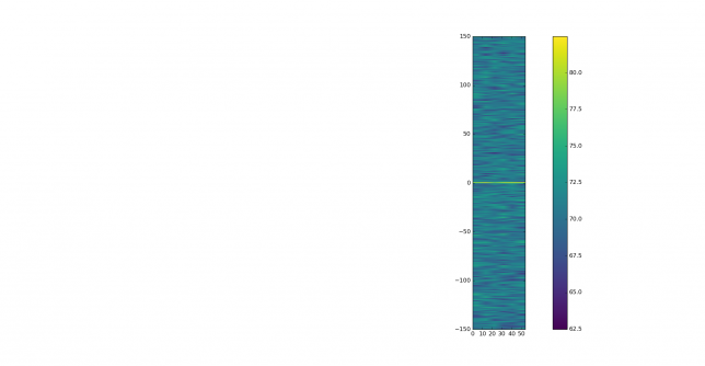
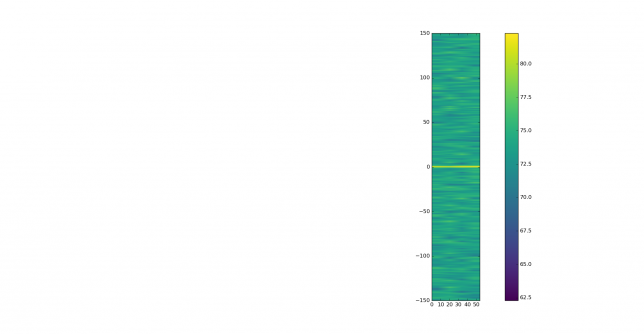
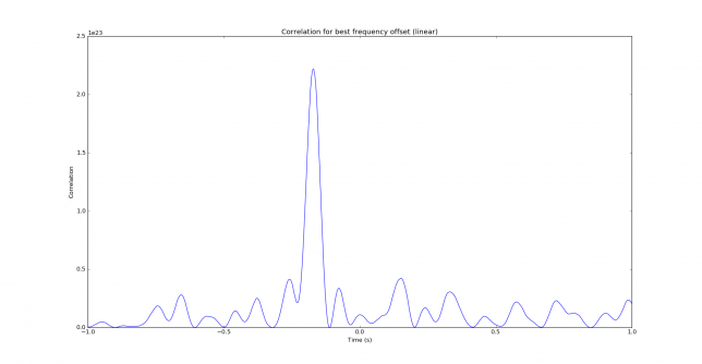
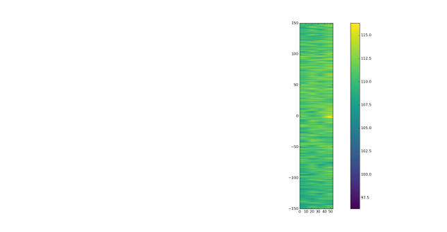
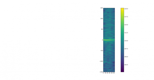
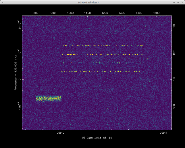
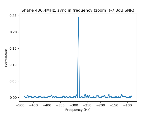
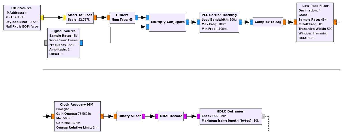
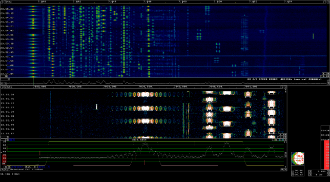
Linrad is used to play the wav recording in CW mode and adequate parameters are set to allow spotting visually in the waterfall signals with inadequate IMD. The parameters are in this gist. The audio output of Linrad is sent into fldigi using snd-aloop. AGC in Linrad is disabled and the audio output level is set low enough to prevent clipping. The BFO in Linrad is set to 1500Hz below the signal, so that the tuned PSK63 signal appears at 1500Hz in fldigi.

The recording is slightly longer than 24 hours, and Linrad-04.12 doesn't like this. In particular, the "Times for playback" screen ('F' key) doesn't work properly. I have patched Linrad to make it work with recordings longer than 24 hours. This is a very simple patch:

--- a/help.c	2017-02-01 00:09:14.000000000 +0100
+++ b/help.c	2017-03-12 16:55:40.119612866 +0100
@@ -200,7 +200,7 @@
 filetime2*=blk_factor;
 filetime2=diskread_timofday1+filetime2/(snd[RXAD].framesize*ui.rx_ad_speed);
 i=rint(filetime2);
-i%=24*3600;
+//i%=24*3600;
 diskread_timofday2=i;
 if(diskread_timofday2 < diskread_timofday1)diskread_timofday2+=24*3600;
 j=i/3600;

Playback is usually done at a fast rate ('F3' key), going to real time only to examine particular stations when distorted signals are spotted. fldigi is used to identify the station by decoding the PSK63 signal and to perform a first measurement of IMD. When a station with inadequately high IMD is found (around -15dB or worse), Linrad is used to save the audio of the signal to a 16bit 48kHz wav file.

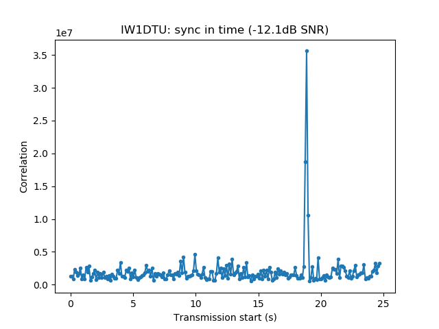
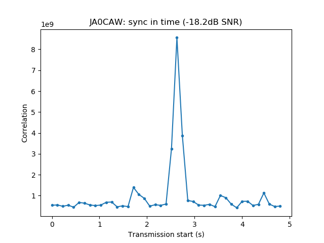
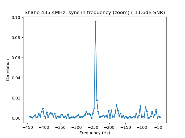
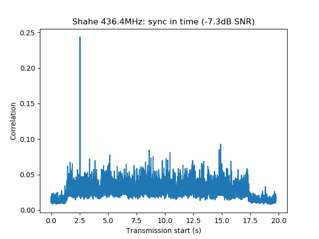
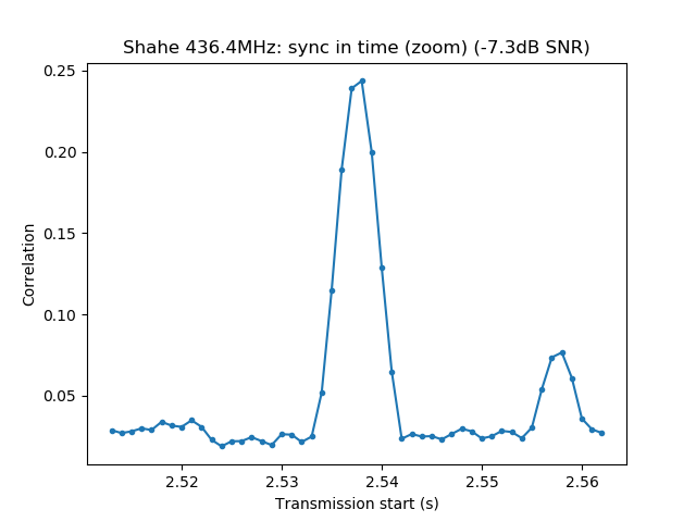
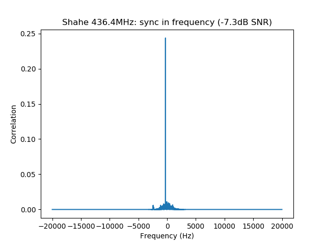
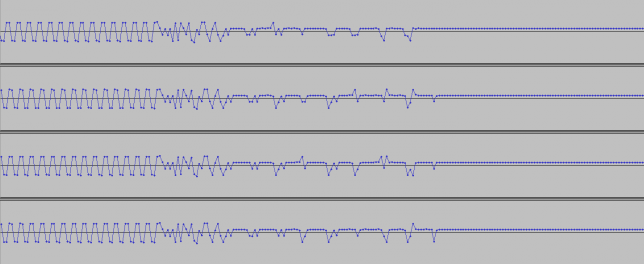
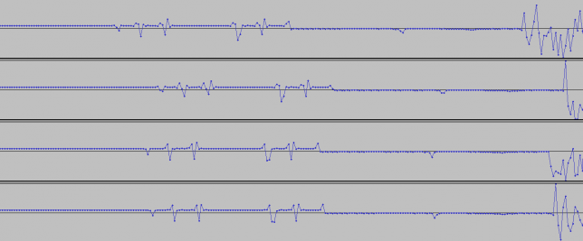
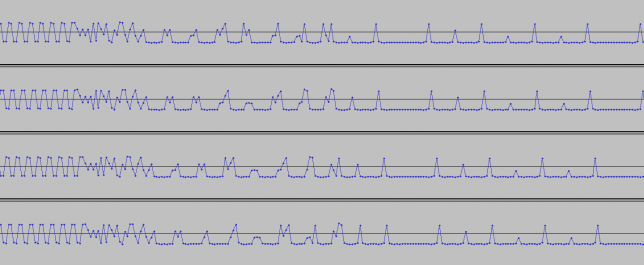
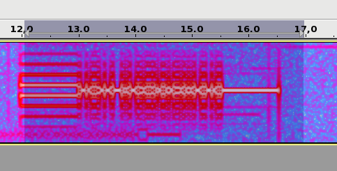
The wav file is then opened with Audacity. It is used to select a short segment of this recording in the following manner. The segment should start with the "sync tones" of the PSK63 signal and contain enough data so that the callsign of the station can be decoded. This is done by cutting just after the signal starts with the "sync tones" and after the transmission stops. By "sync tones" I mean the PSK63 idle signal, which is a repeating sequence of the symbols 0 and 1 and produces a pair of tones spaced 63Hz apart (as well as any intermodulation products). This idle signal is sent for around 1 second before the data starts, to help the receiver synchronized.

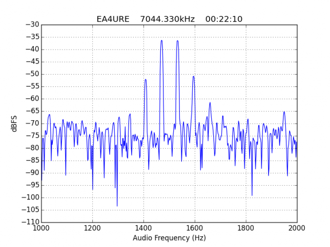
The segment is saved into a 16bit 8000kHz wav file with the name of the station, RF frequency of the PSK63 signal and time within the recording. For instance, ea4ure-7044330-002210.wav is a signal of the station EA4URE, which appeared at 7044.330kHz at 00:22:10 since the start of the recording. The time is approximate, just enough to help one find the signal within the main recording. Note that the gain between the RF input in the Hermes-Lite and this wav file is fixed. There is no AGC anywhere in the processing chain.

The first samples of this wav file are then used to measure IMD (this is the reason why the wav should start with the "sync tones", as we measure IMD on the idle signal). The fil can also be opened with fldigi to check that the station was correctly identified.

IMD measurement

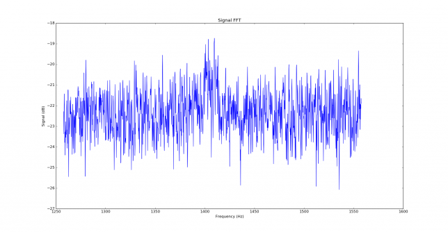
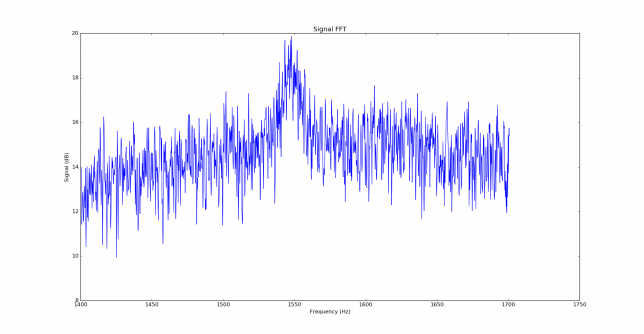
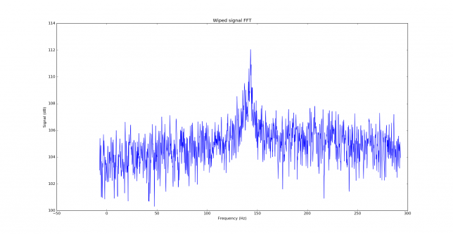
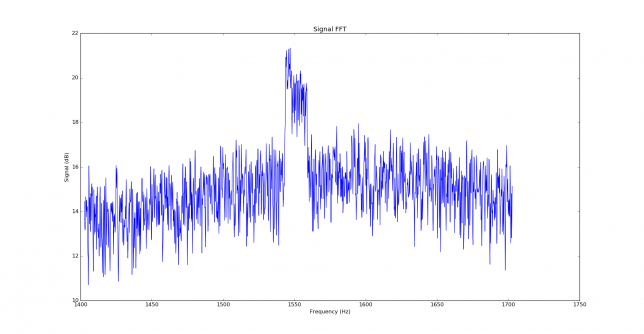
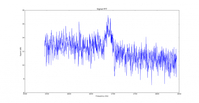
We measure the IMD on the first 4096 samples (512ms) of the 8kHz wav file generated in the previous step. These samples should contain the PSK63 idle signal centred at (or near) 1500Hz. Python is used to compute an FFT and plot the results. A flat top window is used for the FFT computation, because this window has minimal scalloping loss, which is good for this kind of power measurements. The disadvantage of the flat top window is that it has a poor frequency resolution, of around 5 bins. The FFT bins are 1.95Hz wide, so a resolution of 10Hz is acceptable in this context, as we only need to distinguish each of the PSK63 idle tones and their intermodulation products, which are spaced by 63Hz.

The code is as follows:

View the code on Gist.

How to interpret these measurements?

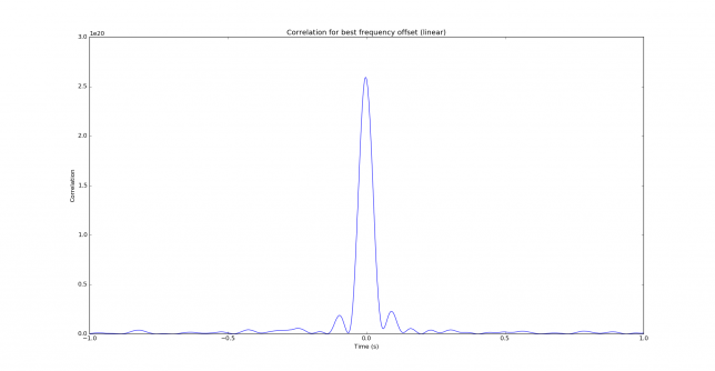
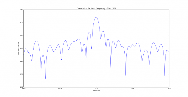
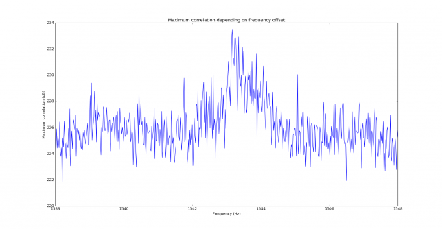
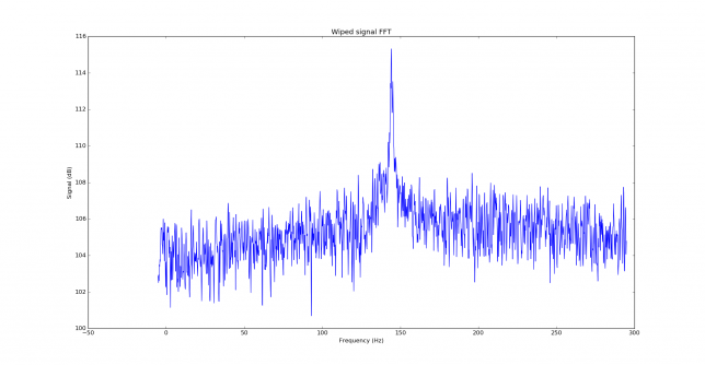
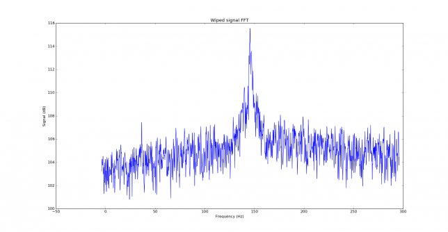
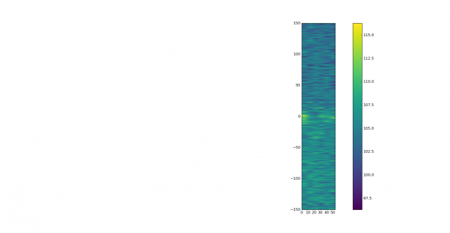
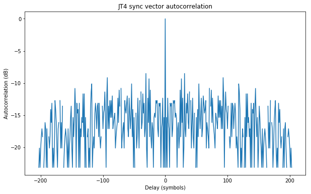
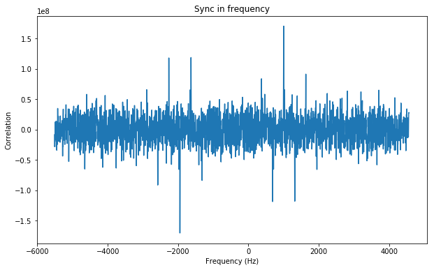
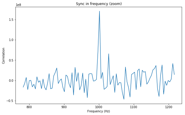
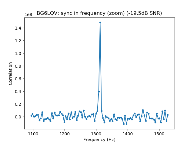
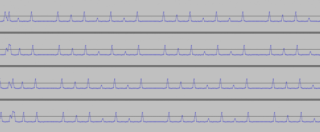
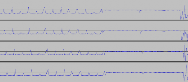
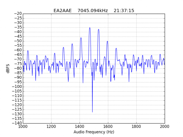
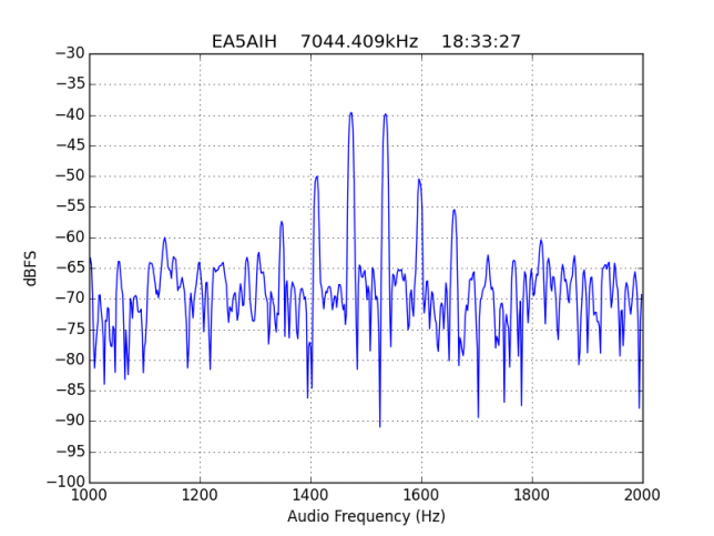
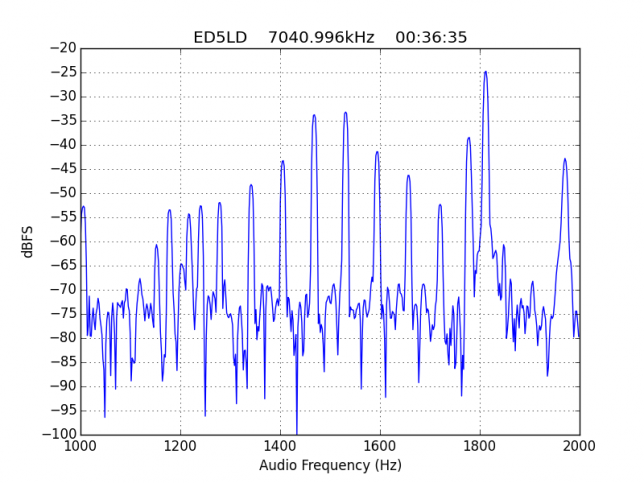
See below for some of the graphs obtained with the IMD measurement Python script. For someone familiar with IMD measurements they should be self-explanatory. The measurement on the PSK63 idle signal is effectively a two-tone test with tones spaced 63Hz and the strength of the different intermodulation products in dB can be read directly from the graph.

If you are new to IMD measurement, the two strong peaks near the centre of the graph represent the strength of the two tones of the signal. The rest of the peaks, which are spaced at constant intervals, are the intermodulation products. The products which are nearest to the two tones in the centre are the third order products, or IM3, the next products going to the sides of the graph are IM5 and so on. The strength of each signal can be read in dB on the y-axis. We are concerned with the difference between each intermodulation product and the main tones. For instance, if the main tones are at -30dB and the IM3 tones are at -45dB, then we say that IM3 is -15db.

What IMD levels are acceptable?

In this document, a description of IMD levels in PSK signals is done. The rule of thumb is that IMD should be -25dB or better, and -20dB is poor performance, -15dB or worse is awful and -30dB or better is excellent. However, this only concerns IM3, which in a properly configured station is the only product strong enough to cause interference.

Recall that a 1dB reduction in output power will usually reduce the order products by dB. Therefore, sending the higher order products many dB's down. Hence, it is very easy to make higher order products disappear by reducing the power a little, while it may not be so easy to get rid of lower order products, especially IM3.

However, higher order products are worse because they broaden the signal bandwidth more, as they are farther apart from the centre frequency of the signal. While a PSK63 should fit in 80 or 100Hz, it definitely has to fit in 500Hz, which is the maximum bandwidth allowed in the digital modes segment of the band plan. In fact, one could argue that products outside a 500Hz bandwidth should be at least 40dB down (which is the requirement for spurious emissions in Spain). For PSK63, this means IM9 and higher order products.

Therefore, as a rule of thumb, we should think that IM3 has to be at least 25dB down, IM5 should be much further down (perhaps 35dB) and IM7 and the rest of the higher order products should be very weak, at least 40dB down and perhaps even 50dB down.

Hall of shame

This is a list of stations showing very bad IMD performance, defined as IM3 around -15dB or worse and/or many strong higher order products. By no means this is a complete study, since only the 40m band has been recorded and when playing back the recording I have just watched the waterfall to judge which stations seemed to have terrible IMD. Remember that to measure the IMD well you need a strong signal or otherwise the intermodulation products will be buried in the noise even if they are not weak enough. Many stations where not strong enough to make measurement possible.

The wav files of all the signals analysed here are in eapsk63-2017-40m-imd.tar.bz2 and can be downloaded in case anyone wants to repeat or check the measurements. Now we pass to the list of all the stations in this hall of shame, together with any additional problems that might give credit for "extra shame". Recall that the time shown in each graph is the time from the start of the main recording, not the time of day.

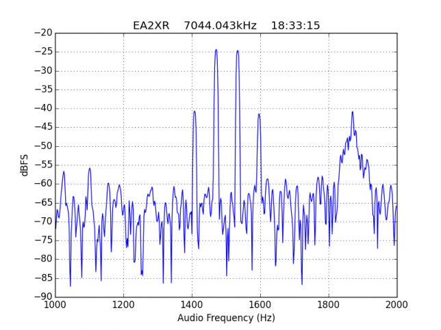
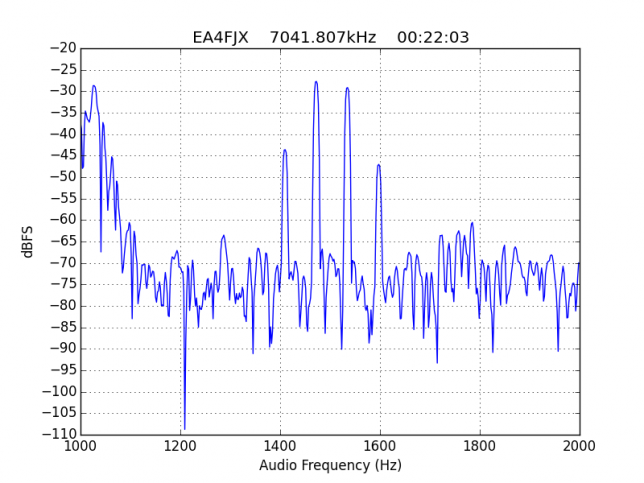
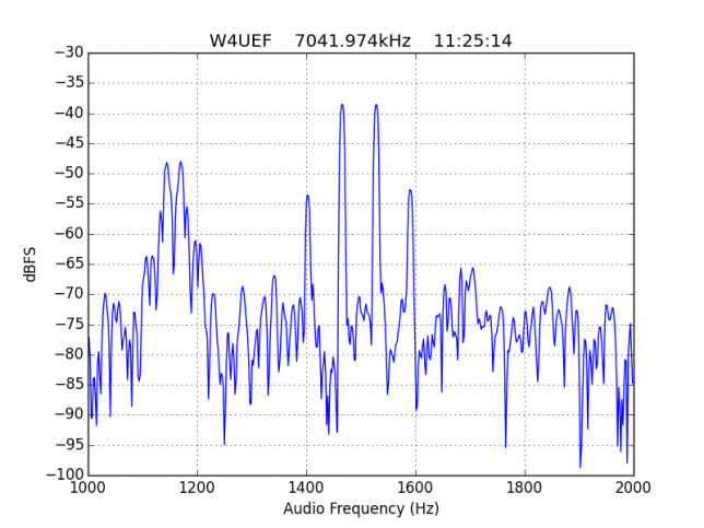
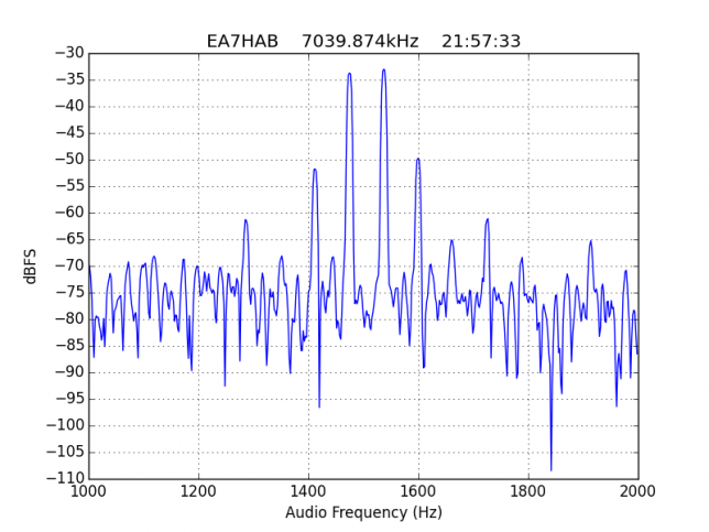
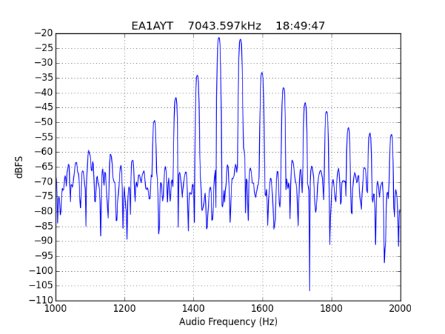
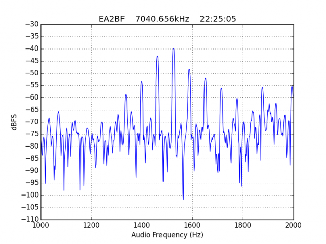
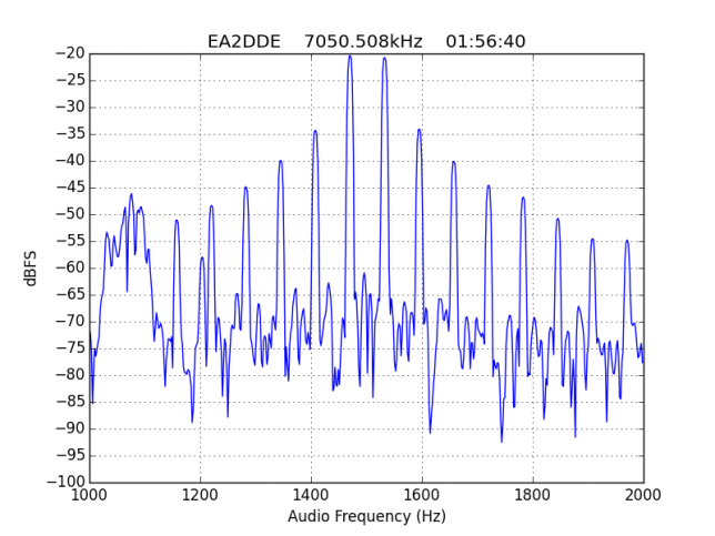
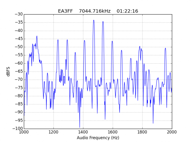
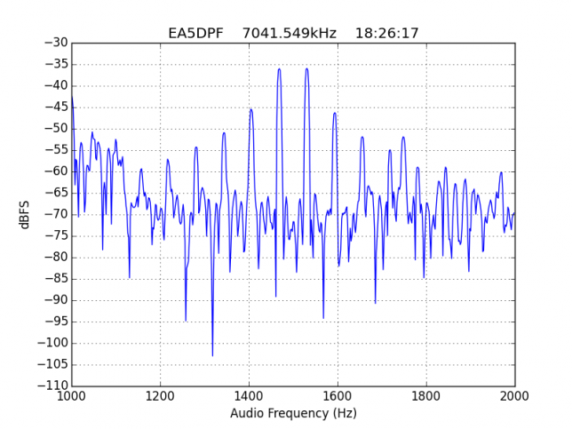
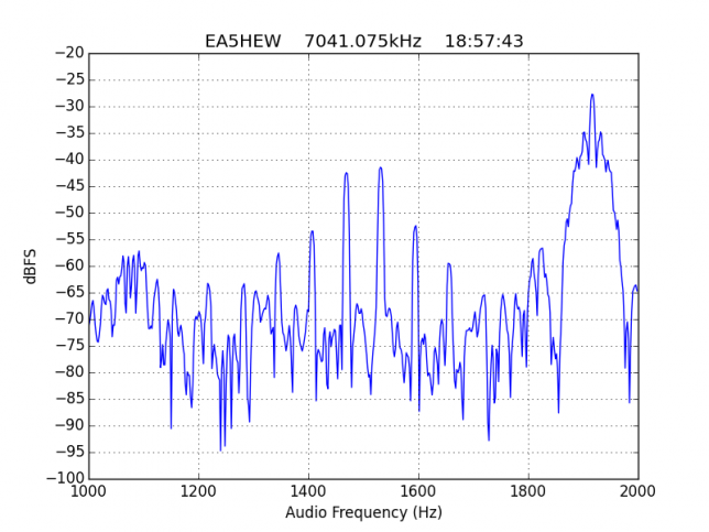
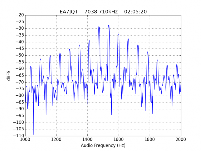
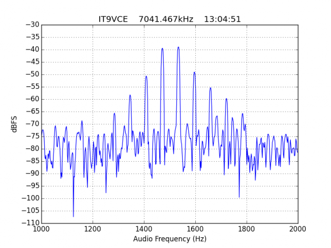
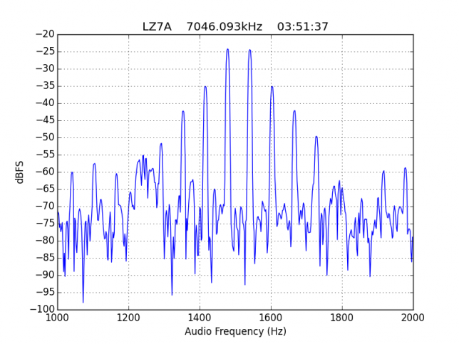
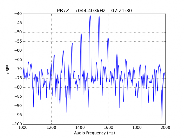
For quick reference, the list of stations in this hall of shame is the following: EA1AYT, EA2AAE, EA2BF, EA2DDE, EA2XR, EA3FF, EA4FJX, EA4URE, EA5AIH, EA5DPF, EA5HEW, EA7HAB, EA7JQT, ED5LD, F5SIZ, IT9VCE, LZ7A, PB7Z, W4UEF.

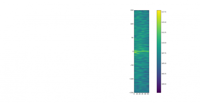
Extra shame for EA4URE, the HQ station of Unión de Radioaficionados Españoles (the Spanish national Amateur society). It plays a special role in the contest as an extra multiplier. In the graph below, it shows significant IMD, with IM3 worse than -15dB. This station should show exemplary operating techniques and technical performance, since it is a symbol of Spanish Amateur radio. The very bad IMD it shows is unacceptable.

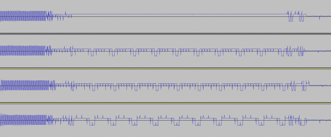
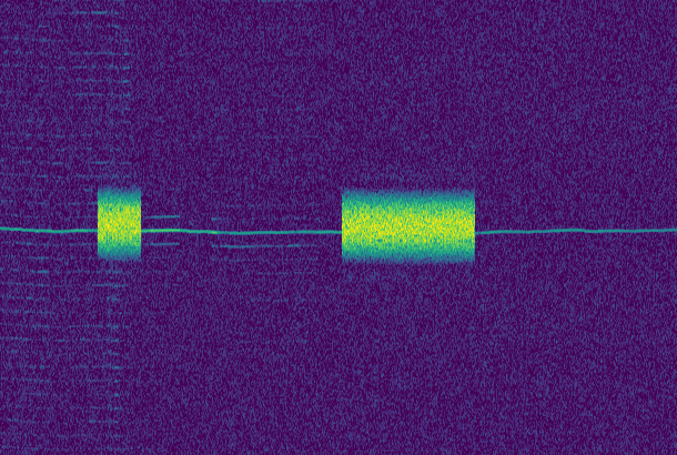
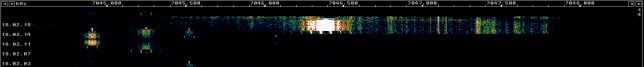
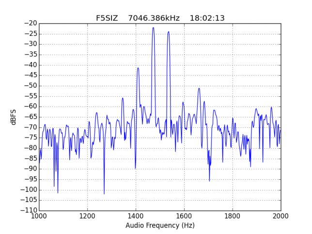
Extra shame for F5SIZ, who not only has a signal which is very unstable in frequency but also puts out all sorts of crap across an SSB transmitter's bandwidth. Its IMD is not so bad but should still be improved.

There are a some stations where only IM3 is strong and the rest of the intermodulation products are weak.

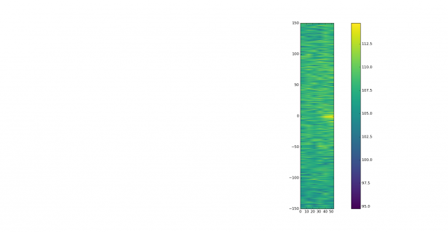
Extra shame for EA7HAB for operating below 7.040kHz, in the segment reserved for CW only. His signal is interesting because IM5 is weak but IM7 is only a bit more than 25dB down.

However, the majority of stations with strong IMD have many strong higher order products, up to IM15. As we have already mentioned, this is completely unacceptable.

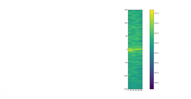
EA2BF is the worst station, with IM3 worse than -10dB.

Extra shame for EA7JQT, for operating below 7.040kHz, in the segment reserved for CW only.

Hall of fame

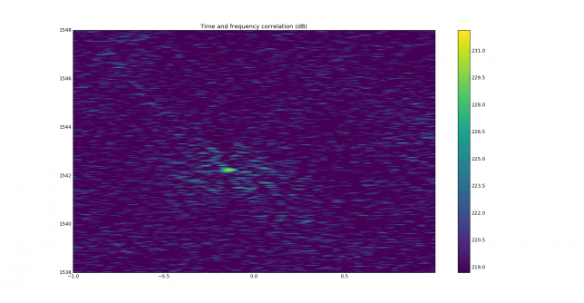
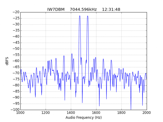
When doing this sort of measurements it is good to process also a clean and strong signal to check that the receive setup is not introducing IMD. When watching the playback, I spotted the following very clean signal, by IW7DBM. IM3, IM5 and IM7 are visible, but all are more than 30dB down, which is excellent. Congratulations. This also shows what is possible with a proper station setup.

I haven't made any special effort to find the cleanest strong signal. This is just something I came across.

What can be done about this problem?

The first thing that one has to do is to note that this is an important problem. Several of the signals shown above contain strong intermodulation products over a bandwidth of nearly 1kHz. Also, many of these stations were calling CQ for several hours, potentially causing interference to many adjacent stations. I think that this post shows enough evidence that IMD levels in PSK contests are terrible and something should be done about it.

The second thing is that every Amateur operator should know how to operate his station properly and take the effort to do so. Probably many of the signals in the hall of shame can be made much better just by adjusting the audio levels properly or changing the transmitter's ALC setup. The most important thing that you should do is to monitor your own signal to measure IMD levels and take action immediately when there is a problem. Very bad IMD is very easy to spot on the waterfall, but you should also make precise measurements to know where you stand. Software for digital modes can be used to measure IMD, but it will usually report IM3 only. Do take care also that the higher order products are way down.

Monitoring your own signal only requires an SSB receiver (which is easy to get these days in the form of a cheap SDR receiver) and the appropriate software. There is no reason why any Amateur should not monitor his own signal. You can also measure IMD over the air, but keep in mind that it can only be measured on a strong signal. If you can't see the intermodulation products on the waterfall then there is nothing you can measure, since the IMD is below the noise floor. Ideally, you should monitor your signal all the time, but at least you should monitor every time you change your station setup, to check that your signal is still clean.

The third thing is that adequate IMD levels should be enforced by the contest rules. A maximum allowable IMD level should be fixed in the contest rules (ideally taking into account products of different order), the organization should monitor the contest and stations not satisfying the IMD limit should be disqualified. There are also other problems which are even more apparent and should not be neglected by the organization: stations transmitting outside the digital modes segment or on top of some well established working frequency for another digital mode, such as the WSPR segment.

If you've read this far, and especially if your callsign appeared in the hall of shame, please do take care that your signal is clean. Don't hesitate to contact me if you need any help in setting up your station properly. Remember that a clean signal makes a more enjoyable experience on the bands for everyone.

Last weekend, I recorded the full EAPSK63 contest in the 40m band with the goal of monitoring IMD levels. I made a 48kHz IQ recording spanning the full 24 contest hours (from 16:00 UTC on Saturday to 16:00 UTC on Sunday). This week I've been playing with making waterfall plots from the recording. These are very interesting, showing patterns in propagation and contest activity. Here I show some of the waterfalls I've obtained, together with the Python code used to compute them.

In all the waterfalls shown here, time is represented in the horizontal axis, and frequency is represented in the vertical axis, with the top of the image corresponding to the highest frequency and the bottom of the image corresponding to the lowest frequency. All the plots are done with FFT transforms overlapping a 50% and the Blackmann window. The banner on top of this post is cropped from a waterfall done with 1024 FFT bins and 4308 averages, thus producing a 1920x1024 image. The resolution is 46.86Hz or 49.96s per pixel.

The image below shows a comparison between the JT65 and JT9 activity and the EAPSK63 contest. It is cropped from a waterfall with 4096 FFT bins and 1077 averages, yielding a 1920x4096 image with a resolution of 11.72Hz or 45.99s per pixel. Remember that you can click on the images to view them in full size.

A large number of the stations participating in the EAPSK63 contest are located in Spain. Hence, their signal is usually strong at my station in Madrid, but late at night this time of the year Spain is in the skip zone for 40m, so Spanish stations are weak or not present at all. Thus, at night only stations elsewhere in Europe and outside Europe are present. The proportions of local and DX stations in the PSK contest and in JT modes are quite different. Also, the patterns of activity throughout the day are different. The JT modes activity depends basically on propagation (people choosing the best bands trying to work DX), while the contest activity has much to do with the local time in Europe. Therefore, we can see really different patterns in the waterfall.

On Saturday night, the JT activity is at its peak, while the contest activity has diminished and is almost non-existent late at night. On Sunday noon, there is strong contest activity, but the JT segment is almost clean and sometimes occupied by SSB stations, since propagation in 40m is too short for DX during the day. The WSPR segment can also be seen near the bottom of the image above. WSRP signals depend almost exclusively on propagation, as activity is roughly constant. However, it is a bit difficult to judge the strength and number of WSPR signals in this waterfall.

The image above was cropped from the following 1920x4096 image. A portion of this image can be cropped to obtain a 1920x1080 image, which can be used as a desktop background.

I have also done a high resolution waterfall with 16384 FFT bins and 29 averages, which yields a 17830x16384 image with a resolution of 2.93Hz or 5.12s per pixel. In this large image, I've found the following interesting regions. All of them are 1920x1080 crops. They are best viewed in full size.

Lots of activity in JT65 and JT9.

A station calling CQ in QRA64A. Unfortunately, no takers. You can also see a JT65 station using the wrong sideband (LSB).

Some stations doing DSSTV using HamDRM, which uses LSB on 40m.

The WSPR segment and the EAPSK63 contest fray, with PSK stations transmitting sometimes on top of the WSPR segment or below 7040kHz.

Two stations using some kind of MFSK digital modes and an SSB station.

The code used to plot the waterfalls in this post is as follows:

View the code on Gist.

This code can be adapted to process any other recordings or for experimenting with different parameters and the EAPSK63 contest recording (perhaps different FFT windows can be tried). It saves the averaged transforms in a file, so computation can be stopped midway and resumed later on or plotting parameters can be changed without having to recompute the FFTs. The waterfall is plotted in PNG chunks to prevent the plotter from running out of RAM. The chunks can be merged later with Imagemagick by doing

convert +append waterfall?.png waterfall.png

In my previous post, I examined a recording of LilacSat-1 transmitting an image. I did some calculations regarding the time it would take to transmit that image and the time that it actually took to transmit, given that the image was interleaved with telemetry packets. I wondered if the downlink KISS stream capacity was being used completely.

You can find more information about the downlink protocol of LilacSat-1 in this post. The important information to know here is that it consists of two interleaved channels: a channel that contains Codec2 frames for the FM/Codec2 repeater and a channel that contains a KISS stream. The KISS stream is sent at 3400bps. At any moment in time, the KISS stream can be either idling, by sending c0 bytes, or transmitting a CSP packet. The CSP packets can be camera packets (which are sent to CSP destination 6) or telemetry packets (and perhaps also other kinds of packets).

I have extracted the KISS stream from the recording and examined its usage to determine if it is being used at its full capacity or if it spends time idling. The image below represents the usage of each byte in the KISS stream, as time progresses. Bytes belonging to image packets are shown in blue, bytes belonging to other packets are shown in red and idle bytes are shown in white. (Remember that you can click the images to view them in full size).

The first 3 or 4 seconds of the graph are garbage, since the signal wasn't strong enough. Then we see some telemetry packets and the image transmission starts. We observe that most image packets are transmitted leaving an idle gap between them. The size of the gap is similar to the size of the image packet. Every 10 seconds, a bunch of telemetry packets are transmitted, in a somewhat different order each time. Some telemetry packets are sent back to back, and others are interleaved with image packets. Image packets are only sent back to back just after a telemetry transmission.

The next graph shows the usage of the KISS stream averaged over periods of 5 secons. The y-axis means fraction of capacity of the link, so a 1 means that the full 3400bps are used. The capacity spent for image packets is shown in blue and the capacity used for telemetry is shown in red. The green curve is the sum of the blue and red, so it means the fraction of time that the link is not idle. We see that the link is never used completely. The total usage ranges between 60% and 90%, but never reaches 100%.

As expected, the capacity used for telemetry spikes up every 10 seconds. The blue curve is more interesting. It is roughly around 55%, but whenever telemetry is sent, it decreases a little. Just after each telemetry burst, the blue curve increases a little. This matches the behaviour we have seen in the previous graph. Every 10 seconds a telemetry burst is sent, using up some capacity that would normally be spent for image. After the telemetry burst, some image packets are sent back to back in a burst, peaking up to 60% capacity, but soon the packets continue being sent with idle gaps between them, and the capacity goes down to 55%.

It is a bit strange that the link is not fully utilised. One would expect that image packets are sent as fast as possible, stopping only to send telemetry. However, we have seen that there are many idle gaps. It seems that the image can't be read very fast or that there is some other throttling mechanism. This would explain why a burst of image packets is sent after each telemetry burst: the image packets buffer up, because the link is sending telemetry. When the link is no longer busy with telemetry, it sends all the buffered image packets in a row, but soon enough image packets can't be produced as fast as the link sends them, so idle gaps appear. This seems quite an important performance issue, as it appears that image transmission speed is capped at about 1870bps.

The Python code that generated these graphs can be seen below. The KISS file is also in the same gist.

View the code on Gist.

The Chang'e 4 is a Chinese lunar mission that will land a rover on the far side of the Moon by the end of 2018. To support this mission, the Chang'e 4 relay satellite will be launched six months before and put into a halo orbit around the Earth-Moon Lagrange L2 point. The relay will provide four 256Kbps links with the rover and lander on X-band and a 2Mbps link with Earth on S-band using a 4.2m dish. Two CE-4 microsatellites will be launched together with the relay satellite. They will be put in a 200km x 9000km lunar elliptical orbit. The main mission of the CE-4 microsatellites is to perform HF interferometry of celestial bodies, using the Moon as a shield from the radiation of the Sun and Earth. The satellites also carry an Amateur radio system called DSLWP, which will provide telecommand, telemetry and image downlink.

A team at Harbin Institute of Technology is currently designing the Amateur radio payload. As it is the case with previous HIT satellites such as BY70-1 and LilacSat-1, the payload will have a camera which can be telecommanded by radio Amateurs, which can use it to take and download pictures. Yesterday, Wei BG2BHC has released some work in progress of the image downlink. Many important parts of the downlink will still change, but releasing the work in progress at this early stage is a very good idea. Probably it is not too late in the development process so that the Amateur community can contribute with ideas and improvements.

The release consists of an IQ recording of the signal containing a full image and a decoder in gr-lilacsat. The IQ recording is at 2ksamp/s, since the signal is FSK at 250baud. Note that the recording is almost 32 minutes long. It takes a while to transmit an image at such a low rate. However, a low baudrate and a good amount of FEC are needed for an effective downlink from the Moon, given the huge path loss of around 197dB in the 70cm band.

The good news about this work in progress is that SSDV is now used to transmit the image. SSDV is a packetised protocol based on JPEG, but which is tolerant to packet loss. In contrast, BY70-1 and LilacSat-1 send JPEG images in 64byte chunks, and a single lost chunk can destroy the image completely. SSDV was originally developed to transmit images from Amateur high altitude ballons, so it is a good idea to use it also for DSLWP.

The bad news is that the way that SSDV has been included into the downlink protocol is not very optimal. In the rest of this post I do an in-depth look at the protocol, point out the main problems and suggest some solutions. Hopefully the protocol can still be modified and improved.

The current downlink protocol of DSLWP is based on the same CCSDS stack using an r=1/2, k=7 convolutional code and Reed-Solomon (255,223) that the rest of the HIT satellites use. In fact, it is very similar to the 4k8 GFSK downlink of LilacSat-2. However, DSLWP uses 250baud GFSK. Wei has already stated that he intends to change GFSK for GMSK with coherent receiving and the convolutional code by a Turbo code. He also said that he will design a new packet header, although it is not clear what he has in mind.

In the following, I will describe the protocol from the point of view of the transmitter. There are 3 independent KISS streams, which are called virtual channels. All the packets from DSLWP are 223 bytes long. They contain a 5 byte header, whose contents are specified in dslwp_tm_header.h, and 218 bytes from one of the 3 virtual channels (the header states which channel). The 223 byte packets are encoded with the CCSDS Reed-Solomon (255, 223) code using the conventional basis and scrambled with the CCSDS synchronous scrambler. Then the CCSDS 32-bit syncword 0x1acffc1d is added in front of the packet and the packets are sent through the CCSDS r=1/2, k=7 convolutional encoder (following the CCSDS/NASA-GSFC convention for the polynomials). The output of the convolutional encoder is sent as 250baud GFSK.

In the sample recording by Wei, the SSDV packets corresponding to the image are sent in the second virtual channel. They are sent in a consecutive manner, leaving only two c0 bytes between them (c0 is the frame delimiter or idle marker in the KISS protocol). There are a total of 95 SSDV packets. I have saved the packets in the file ssdv.bin. This file can be decoded with SSDV to produce the JPEG image below. It is a 640 x 480 image and its size is 20056 bytes.

SSDV packets are always 256 bytes long, so the SSDV packets amount to a total of 24320 bytes. This is a reasonable overhead to pay, since the SSDV packets include 32 bytes of Reed-Solomon check bytes, which accounts for most of this overhead.

The main problem that I find with the current protocol is that the SSDV packets, which are 256 bytes long and include their own Reed-Solomon FEC, do not fit well within the scheme of sending a KISS stream by chunks of 218 bytes. Since the DSLWP packets are also protected by Reed-Solomon, there are two independent layers of Reed-Solomon FEC. This adds an unreasonable amount of overhead and doesn't provide much extra protection (on the other hand, a concatenated code with a convolutional code and Reed-Solomon is usually a good idea). Also, since SSDV packets are slightly larger than the KISS stream chunks, each SSDV packet is sent inside two or three DSLWP packets. This means that if a DSLWP packet is lost, we will usually lose two SSDV packets, since in general a DSLWP packet contains bytes from two different SSDV packets.

For the best performance, SSDV packets should not be fragmented. If they need to be fragmented, each fragment should contain bytes from only one SSDV packet. Also, there should be a single layer of Reed-Solomon FEC.

In the recording, a total of 114 DSLWP packets were sent. Since each packet is 259 bytes long (counting the CCSDS syncword), this amounts to 29526 bytes, which is an overhead of 21.4% in comparison with the SSDV packets alone. Since the bit rate is already quite low, the overhead should be as low as possible. An overhead of 20% is too much.

There are many different ways in which the current protocol can be improved. Ideally, we would like to send SSDV packets without fragmentation and as little overhead as possible. A simple idea is to attach the CCSDS syncword in front of each SSDV packet and send these packets through the convolutional encoder. Optionally, each SSDV packet can be scrambled with the CCSDS scrambler. However, it is necessary to study whether scrambling provides any advantage. The drawback of the scrambler is that it transforms each bit error uncorrected by the Viterbi decoder into three byte errors for the Reed-Solomon decoder. Probably, since most of the contents of an SSDV packet is scan data from a JPEG file, the data is random enough that a scrambler is not necessary.

This approach doesn't preclude the possibility of sending telemetry and other data using the current protocol. SSDV packets (perhaps unscrambled) and scrambled DSWLP packets with their Reed-Solomon FEC can both be sent without any type marker, since the SSDV decoder and the DSWLP Reed-Solomon decoder will reject packets of the other type.

A very small improvement can also be gained if one notes that it is not necessary to send the first byte of each SSDV packet over the air. This byte is always 0x55 and it serves as a sync byte. In our case, we are using CCSDS syncword, so it is not necessary to send the sync byte. The receiver can insert it later, before passing the packets to the SSDV decoder.

Also, one should note that the SSDV protocols supports uncoded packets. In this mode, no FEC is used, and instead there are 32 extra bytes for JPEG scan data. Uncoded SSDV therefore adds very little overhead to the original JPEG file. It makes sense to use uncoded SSDV if one wishes to replace the Reed-Solomon (255,223) code by another outer code. In this case, the uncoded SSDV packets would be encoded by the outer code and then passed to the convolutional encoder, together with their syncword. Probably uncoded SSDV shouldn't be used with a convolutional code alone, since the Viterbi decoder can still leave some remaining bit errors and the SSDV decoder rejects any packet with incorrect CRC32. However, if the convolutional code is replaced by a code with better performance, then it can also be a good idea to use uncoded SSDV.

I can't talk about SSDV and FEC without mentioning Wenet from Project Horus. This is a 115kbps FSK modem for Amateur high altitude balloons which sends SSDV images using an LDPC code. This project is definitely worth looking at carefully. Perhaps it's not necessary to reinvent the wheel for DSLWP and an adaptation of Wenet will perform well.

I have added a decoder for the DSWLP test recording to gr-satellites. The main improvement of my decoder compared to the decoder in gr-lilacsat is that it uses soft Viterbi decoding, which improves the BER performance noticeably. Still, this is not a fully functioning decoder. The SSDV decoder expects complete SSDV packets on its input. If a DSWLP packet is lost, then a partial fragment of an SSDV packet is stored in the output file and the SSDV decoder complains. A tool that only passes complete SSDV packets to the decoder will be needed.

Several weeks ago, in an AMSAT EA informal meeting, Eduardo EA3GHS wondered about the possibility of using WSJT-X modes through linear transponder satellites in low Earth orbit. Of course, computer Doppler correction is a must, but even under the best circumstances we cannot assume a perfect Doppler correction. First, there are errors in the Doppler computation because the TLEs used are always measured at an earlier time and do not reflect exactly the current state of the satellite. This was the aspect that Eduardo was studying. Second, there are also errors because the computer clock is not perfect. Even a 10ms error in the computer clock can produce a noticeable error in the Doppler computation. Also, usually there is a delay between the time that the RF signal reaches the antenna and the time that the Doppler correction is computed for and applied to the signal, especially if using SDR hardware, which can have large buffers for the signal. This delay can be measured and compensated in the Doppler calculation, but this is usually not done.

Here we look at errors of the second kind. We denote by the function describing the Doppler frequency, where is the time when the signal arrives at the antenna. We assume that the correction is not done using , but rather , where is a small constant. Thus, a residual Doppler is still present in the received signal. We will study this residual Doppler and how tolerant to it are several WSJT-X modes, depending on the value of .

The dependence of Doppler on the age of the TLEs will be studied in a later post, but it is worthy to note that the largest error made by using old TLEs is in the along-track position of the satellite, and that this effect is well modelled by offsetting the Doppler curve in time. This justifies the study of the residual Doppler .

In this study, we will use the satellite LilacSat-1, which is a member of the QB50 constellation. It was released from the ISS on May 25 this year, and so it is in a circular orbit with an altitude of around 420km and inclination of 52º. The TLE used is

1 42725U 98067ME  17188.90653574  .00007620  00000-0  11662-3 0  9998
2 42725  51.6409 294.7316 0007224  26.7821 333.3542 15.55427837  6725

This was the latest TLE available from Celestrak for LilacSat-1 at the time when this research was started. The epoch is 2017/07/07 19:45:24. We will be looking at the pass starting at 2017/7/9 03:12:00 UTC, which is the next overhead pass at the time when this research started, as seen from my station's location at 40.6007, -3.7080, 700m ASL. This is how this pass looks like in Gpredict.

The Doppler, and especially the rate of change of Doppler near the time of closest approach is higher in a high elevation pass, so this overhead pass was chosen to provide a worst case. We will only look at the effect of the Doppler in the downlink of the satellite. This case is interesting if the residual Doppler in the uplink is much smaller than the residual Doppler in the downlink, or if the signal is transmitted by the satellite as a beacon. In the next post we will look at both the uplink and downlink Doppler, as this case is much more involved, since it depends on the geometry between the two stations and the satellite.

The most popular bands used in linear transponder satellites are the 2m band and the 70cm band. Here we will study the 70cm band, since the Doppler is higher. The 2m band is essentially 3 times "easier". We assume a frequency of 436.5MHz, which is in the middle of the 70cm satellite sub-band (435-438MHz).

We will use PyEphem to perform the Doppler calculations in Python, by calculating the range velocity (change of distance to the satellite with respect to time). It was verified that Gpredict and PyEphem give the same values for the range velocity, as there are some worrying reports that PyEphem computes a wrong range velocity. The Doppler profile for this pass can be seen below.

As expected for a low Earth orbit satellite pass on the 70cm band, the Doppler goes down from 10kHz to -10kHz. The most challenging part for Doppler correction is near the time of closest approach, when the Doppler passes through 0Hz, the derivative of the Doppler is largest, and its second derivative changes sign.

Now we turn to the residual Doppler . Note that this can be approximated by for small delta. Below we can see the residual Doppler computed for different values of .

We note that the shape of the residual Doppler is always the shape of the derivative . Positive residual Dopplers correspond to the case , since . We also note that even for an offset as small as 200ms, the residual Doppler is already around 35Hz at the time of closest approach. This can be devastating for many WSJT-X modes, which have tone spacings much smaller than 35Hz. We remark that several WSJT-X modes are able to compensate some form of linear frequency drift. However, near the time of closest approach this is not very helpful. Perhaps much better performance can be achieved by trying to compensate for a frequency drift given by a second order polynomial, but probably this already makes the search space too large.

We see that outside of the interval we can ignore the residual Doppler for the values of that we are considering here. The residual Doppler is small and more or less linear. This is encouraging: only the 3 central minutes of the pass are challenging. Here we only look at these 3 central minutes, and we decide to start all our WSJT-X signals at , where the residual Doppler is worst (note that all the modes that will be examined here use periods of 60 seconds, except FT8, which uses periods of 15 seconds).

The decoding tests with WSJT-X have been made with Python. As stated above, PyEphem is used for the Doppler computations, while NumPy is used for DSP computations. The residual Doppler is computed using PyEphem for using a step of 1 millisecond. Then the command line tools from WSJT-X are used to generate WAV files with the signals at a given SNR. These WAV files are read with NumPy, shifted in frequency according to the residual Doppler and stored in disk again. Finally, they are passed to the WSJT-X command line decoder and the number of decodes depending on is noted. There is more information about generation of sample signals and decoding using the WSJT-X command line tools in this post. The version of WSJT-X used is r8021 from SVN.

The DSP algorithm used to shift in frequency is as follows. A complex sinusoidal oscillator is generated using the residual Doppler frequency. The samples from the WAV file are passed through a Hilbert transform filter and multiplied by the oscillator. Then the real part is taken.

We have studied the following WSJT-X modes:

• JT9A. This is the most sensitive 1 minute mode. It is intended for HF and it is very narrow (15.6Hz, tone spacing 1.736Hz). It is expected that this mode is the worst performer regarding residual Doppler.
• QRA64A. This mode is intended as a replacement for JT65B in EME and also for terrestrial use in VHF, UHF and perhaps the lower microwave bands. The bandwidth is 111.1Hz and tone separation is 1.736Hz. It is designed with Doppler spreading caused by lunar libration in mind. This may help it resist residual Doppler.
• QRA64C. It is the same as QRA64A but with a larger tone spacing, which makes it suitable for EME and some forms of terrestrial propagation in the microwave bands. The bandwidth is 439.2Hz and tone spacing is 6.944Hz. The larger tone separation may help it resist residual Doppler better than QRA64A.
• QRA64E. It is the widest QRA64 mode, with a bandwidth of 1751.7Hz and tone spacing of 6.944Hz.
• FT8. This is a new 15 second mode intended for fast changing conditions such as Es in 6m. It has quickly gained a lot of popularity in HF. It trades off sensitivity by the shorter period. The bandwidth is 50Hz and tone separation is 6.25Hz. The shorter transmit period could help resist residual Doppler, since the total change in Doppler during the period is smaller.
• JT4G. This mode is intended for microwave propagation forms with lots of Doppler spread, such as rain scatter. The bandwidth is 949.4Hz and the tone separation 315Hz. Note that, in contrast to the other modes we are studying, the tone separation of JT4G is much larger than the maximum residual Doppler that we are considering.

More information about these and other WSJT-X modes can be found in Table 3 in the WSJT-X User Guide. It would have been interesting to study JT9H also, which is a very wide variant of JT9A. Unfortunately it seems that there are no command line tools to generate signals of JT9 submodes B through H.

Since the JT9A signal is very narrow and the command line tools support it, to test JT9A we generate a WAV file with 25 JT9A signals at different frequencies. The remaining modes are too wide or the command line tools do not support generation or decoding of multiple signals properly. Thus, 10 separate WAV files with a single signal in each one are generated.

When doing the simulations, we have noted that there is a decoding threshold for the offset . When is greater than this threshold, none or very few decodes are produced. If is smaller than the threshold, then all or almost all of the signals are decoded. The threshold is dependent on the mode, but we have found that it also depends on the SNR of the signals. For a fixed mode, the threshold might be larger for stronger signals.

Thus, we consider three cases for the SNR. First, a low SNR, which is a couple of dBs above the decoding threshold of the mode. Second, -20dB SNR, which is above the decoding threshold for most of the modes studied. Third, -15dB SNR. For an SNR much higher than -15dB, the signals are not weak any more and it may make sense to use other kinds of modes not specialized in weak signals.

The results for the threshold (in seconds) depending on the mode and SNR are summarised in the table below.

Note that the low SNR for FT8 is defined as -18dB, since in fact no decodes were obtained at -20dB SNR.

The basic idea of building a WSJT-X decoder that can operate through low Earth orbit linear transponders is to do a search in the offset until a decode is achieved. In this manner, we try to compensate for the unknown residual Doppler. This will be treated more in depth in a future post. Modes with lower threshold need to have a larger search space, since more values for the offset need to be tried. This increases the computation time.

In view of the table above, we see that JT9A is not a very good idea, since it is not very tolerant of residual Doppler. Surprisingly, JT4G is not a very good performer either if we take into account that its tone spacing is very wide. QRA64E seems a good performer, and its sensitivity is almost as good as QRA64A. Another interesting mode is FT8. Its threshold improves a lot with a better SNR and its 15s period makes it easier to send several messages during a 10 minute pass. Therefore, for the next studies we will centre our attention in QRA64E and FT8. For these modes, it seems that it is acceptable to search for in steps of 0.2 seconds (perhaps even 0.3 seconds).

Python code. The Python code used in the preparation of this article can be found in this gist.

Acknowledgements. I must thank Eduardo EA3GHS for introducing me to this beautiful and exciting problem and also for his detailed presentation of simulations of Doppler curves using TLEs of different age. His convincing presentation motivated this work.

Lately, I have been playing around with the concept of doing acquisition and wipeoff of JT9A signals, using a locally generated replica when the transmitted message is known. These are concepts and terminologies that come from GNSS signal processing, but they can applied to many other cases.

In GNSS, most of the systems transmit a known spreading sequence using BPSK. When the signal arrives to the receiver, the frequency offset (given by Doppler and clock error) and delay are unknown. The receiver runs a search correlating against a locally generated replica signal which uses the same spreading sequence. The correlation will peak for the correct values of frequency offset and delay. The receiver then mixes the incoming signal with the replica to remove the DSSS modulation, so that only the data bits that carry the navigation message remain. This process can be understood as a matched filter that removes a lot of noise bandwidth. The procedure is called code wipeoff.

The same ideas can be applied to almost any kind of signal. A JT9A signal is a 9-FSK signal, so when trying to do an FFT to visually detect the signal in a spectrum display, the energy of the signal spreads over several bins and we lose SNR. We can generate a replica JT9A signal carrying the same message and at the same temporal delay than the signal we want to detect. Then we mix the signal with the complex conjugate of the replica. The result is a CW tone at the difference of frequencies of both signals, which we call wiped signal. This is much easier to detect in an FFT, because all the energy is concentrated in a single bin. Here I look at the procedure in detail and show an application with real world signals. Recordings and a Python script are included.

As an example, the image below shows the FFT of a JT9A signal at -27dB SNR in AWGN (over a 2500Hz bandwidth). The signal is at 1400Hz, but it is barely visible.

The parameters used for this FFT are a sampling rate of 12000Hz, FFT length of samples, Blackman window, transforms overlapping 50%.

Below we can see the wiped signal. It is around 11dB over the noise floor. The parameters for the FFT are the same as above.

Before looking at correlations between the signal and replica, it is usual to look at the autocorrelation of the replica, to see what properties it has. First we show the FFT of the replica. We can see that a JT9A signal is 15.6Hz wide, so it spreads over many FFT bins. Each FFT bin is 0.18Hz wide, so the signal spreads over 85 bins. After wiping off, we concentrate all the power in a single bin, obtaining an large increase in SNR.

The correlation is performed both in frequency and time. In fact, only the time offset is needed to perform wipeoff, but to obtain the time offset, first the frequency offset must be found, since time correlation only works properly when the frequency offset is known. The figure below shows the maximum of the correlation in time for each frequency offset. By peaking this maximum we find the correct frequency offset. In this case, the signal has been found at 1400Hz, which is the frequency we are using for the replica. We note that the sidelobes in the figure below are 11.5dB down.

The two figures below shows the correlation in time for the correct frequency offset, in a linear and dB scale. We see that not a lot of temporal resolution is provided by JT9A. This is expected, since the keying rate is rather low. The peak is 3dB down at 29ms time offset, so the temporal resolution given by correlation is on the order of 60ms. This corresponds to 18000km, so multipath cannot be seen by studying the correlation in time.

Still, it is interesting that an m-FSK signal such as JT9A improves the resolution in time. In contrast, an unfiltered BPSK signal carrying a PRN sequence has a resolution in time on the order of the inverse of the baudrate, which for JT9A is 576ms.

Finally we show the autocorrelation in frequency and time. We can see that, although resolution in time is poor, the resolution in frequency is rather good, and in fact for the correct time offset, the autocorrelation has a very sharp response in the frequency parameter.

Now we show the correlation plots for the -27dB SNR signal over AWGN. They are essentially the same as the autocorrelation of the replica, but with added noise.

To study time-varying signals, such as signals with fading or frequency drift, a waterfall is quite useful. The figure below shows the waterfall for our -27dB SNR signal. It is barely visible. The parameters are an FFT size of , Blackman window, transform overlap of 50% and 6 averaged transforms per waterfall line. The dynamic range is 20dB.

The wiped signal is clearly visible in the waterfall below, which was computed with the parameters given above.

For signals having large frequency spread it is sometimes useful to compute a waterfall with a coarser resolution in frequency, using an FFT size of , Blackman window, transform overlap of 50% and 16 averaged transforms per waterfall line. The dynamic range is also 20dB.

While this procedure works beautifully with ideal signals such as our -27dB SNR over AWGN signal, real world signals have multipath, Doppler spread, phase noise and all sorts of things. These factors make the correlation more difficult by spreading the correlation peak. Also, after wipeoff, the wiped signal inherits all the spectral properties from the original signal. For instance, if the original signal drifts in frequency, the wiped signal will also drift in frequency in the same way.

This is interesting because it can serve as a way to analyse the propagation path: Doppler spread can be judged better on a single tone in the wiped signal, reflections off aircraft scatter are visible by their Doppler shift in the wiped signal and so on. In fact, this is one of the practical applications that I see for these techniques. On August 5, Iban EB3FRN and I were doing some tests with JT9A over a 403km path in the 2m and 70cm bands. We were not quite sure if we were hearing each other by tropospheric scatter or by aircraft scatter. This is what motivated this research.

Another application is to detect visually the presence of JT9A signals which are a few dB below the decoding threshold. This indicates whether a QSO could be possible if conditions improve slightly. By correlating against the known transmitted message, a large improvement in SNR is obtained.

As a real world example, I am using the signals I received from EB3FRN on August 5. We managed a QSO in 2m quite easily, while in 70cm we couldn't do it, because I only managed to hear Iban once (while he was hearing me most of the time). The first signal decoded from Iban in 2m was at 11:01, with the message "EA4GPZ EB3FRN JN01". The signal is visible in the FFT plot.

The correlation in frequency produces lots of responses caused by Doppler spread and possibly aircraft scatter reflections.

In the time and frequency plot we can see that the main correlation peak is smeared, while there are several other correlation peaks. These should be discarded, as the difference in time delay is too large and not compatible with any multipath that may happen over a 400km path.

The FFT of the wiped signal shows frequency spread, most likely given by the tropospheric scatter, and responses at some frequencies that might come from aircraft scatter reflections. These are best seen in the waterfall plots.

The waterfall plot of the original signal doesn't show much, except for a strong signal between 0 and 10 seconds, slightly lower in frequency than the main signal.

This strong signal can be seen better in the waterfall of the wiped signal. It probably comes from aircraft scatter. The main tropospheric signal can be seen drifting down in frequency slightly, while one can discern two individual reflections at lower frequencies.

These are best seen in the coarse waterfall.

The next signal, at 11:03 didn't decode, but it shows good correlation against the message "EA4GPZ EB3FRN JN01". We show the time and frequency correlation and the waterfalls for the wiped signal. It is apparent that the signal was only present for the last 15 seconds of the period, probably received from aircraft scatter.

The signal at 11:05 is the strongest and cleanest signal received. We show the signal FFT, time and frequency correlation, FFT of the wiped signal, waterfall of the signal, and the two waterfalls of the wiped signal.

Below we show the wiped signal corresponding to 11:07, which carries the message "EA4GPZ EB3FRN R-27".

Next, at 11:15 we have "EA4GPZ EB3FRN RRR".

At 11:17 we have "EA4GPZ EB3FRN 73". This signal is strong and interesting, because the FFT of the wiped signal shows a peak 60Hz below the main signal. This could correspond to an aircraft scatter reflection, as 60Hz of Doppler corresponds to around 450km/h. However, this peak is not visible in the waterfall, perhaps because the reflection had a short duration.

At 11:41 we have the only signal that I managed to copy in 70cm. The message is EA4GPZ EB3FRN -22. We show the signal FFT, time and frequency correlation, wiped signal FFT and signal and wiped signal waterfalls. The correlation is quite smeared, the wiped signal is almost as wide as the original signal and the signal is only easily visible during the first 15 seconds, so it seems amazing that WSJT-X can decode this signal.

The SNR in these recordings is not so strong as to bring out all the details of the propagation path. Doing the same experiment with much stronger signals will probably show some interesting details of the Doppler spread caused by tropospheric scatter and perhaps bring out weak aircraft scatter reflections.

The WAV recordings used in this post can be downloaded here (84MB). The Python code I have used is in this gist. The script wipeoff.py can be used in two ways. First, as

wipeoff.py 170805_1101.wav

it will use jt9 to decode the file and get the message and a coarse frequency estimate for the signal. This can be used with files that jt9 is able to decode. If jt9 is not able to decode a file but the message and coarse frequency are known, wipeoff.py can be run as

wipeoff.py 170805_1101.wav 1543 "EA4GPZ EB3FRN JN01"

to get these parameters directly from the command line. The coarse frequency needs to have an accuracy of 5Hz.

This is a follow-up to the part I post about using WSJT-X modes through a linear transponder on a LEO satellite. In part I, we considered the tolerance of several WSJT-X modes to the residual Doppler produced by a temporal offset in the Doppler computation used for computer Doppler correction. There, we introduced a parameter which represents the time shift between the real Doppler curve and the computed Doppler curve. The main idea was that a decoder could try to correct the residual Doppler by trying several values of until a decode is produced.

Here we examine the effect of TLE age on the accuracy of the Doppler computation. The problem is that, when a satellite pass occurs, TLEs have been calculated at an epoch in the past, so there is an error between the actual Doppler curve and the Doppler curve predicted by the TLEs. We show that the actual Doppler curve is very well approximated by applying a time shift to the Doppler curve predicted by the TLEs, justifying the study in part I.

We look at the same pass that we studied in part I: the 2017/7/9 03:12:00 UTC pass of LilacSat-1 over my station (40.6007, -3.7080, 700m ASL). The TLE in Space-Track whose epoch is nearest to the time of the pass is

1 42725U 98067ME  17189.87025697 +.00007644 +00000-0 +11689-3 0  9999
2 42725 051.6407 289.9183 0007265 030.1333 330.0075 15.55443398006852

Note that this TLE is different from the one used in part I. Presumably, this TLE wasn't available yet when I started writing part I. We will assume that this TLE predicts the actual Doppler curve. Actually, this TLE was measured 6 hours and 23 minutes before the pass.

Typically, we don't have access to such a current TLE during the time of the pass, so we have to do our Doppler prediction using an older TLE. For instance, when I started writing part I, the TLE I used was the most current and it had an epoch of 2017/07/07 19:45:24. The pass I selected was the next overhead pass over my station.

Now let us look at the problem of predicting the Doppler with an older TLE. To exaggerate the effects, I have selected the TLE

1 42725U 98067ME  17183.50952476 +.00011042 +00000-0 +16628-3 0  9992
2 42725 051.6406 321.6862 0006959 008.0741 352.0361 15.55338480005862

which was measured 6 days and 9 hours before the TLE I am taking as current. The figure below shows the different downlink Doppler curves. The downlink frequency is taken as 436.5MHz, in the middle of the 70cm Amateur satellite band.

We can see that the actual Doppler curve looks very much like a time shifted version of the predicted Doppler curve. Therefore, applying an adequate time shift to the predicted curve yields a very good approximation of the actual Doppler. A simple way to compute this is as the difference between the times where each Doppler curve is zero (which correspond to the times of closes approach). This difference, called "best delay", is 7.38 seconds in this case. In the figure below we see that the difference between the actual Doppler and the predicted Doppler shifted by 7.38 seconds is only of a few Hz.

A decoder trying to correct the residual Doppler will test different values of until a decode is produced. The thresholds obtained in part I show how precise the search for the correct needs to be depending on the mode.

To study the effect of TLE age in the Doppler prediction, we compute the best delay for all the TLEs in Space-Track taken during the week before the pass. The results are shown in the figures below. The second figure is just a zoomed-in portion of the first figure.

These figures are very interesting. The difference in best delay between two consecutive points is a measure of how much the TLE parameters are changing because the orbit of the satellite deviates from the prediction done by the SGP model. We see that sometimes the satellite deviates much from the SGP model, causing changes of several seconds in the best delay, while other times the changes in the best delay are small. These effects should be studied for several satellites over longer time spans. Perhaps I'll do it in a future post.

The conclusion of these figures is that sometimes the best delay can be on the order of several seconds, perhaps as high as 10 seconds. However, many times, if using the latest TLEs available, the best delay will be on the order of a few hundreds of ms. This means that it is possible for a decoder to try in real time different values of until a decode is found. For instance, if using FT8, a step of 0.25 seconds in the search for can be used.

The figure below shows the residual downlink Doppler when correcting each of the old TLEs with the best delay computed above. The age of the TLEs is encoded using the inferno colormap, with older TLEs in black and newer TLEs in yellow. We see that the residual Doppler is very small in all cases. This means that most of the error produced by using older TLEs happens in the along-orbit component of the position of the satellite.

So far we have only concerned ourselves with the downlink Doppler. A strategy to deal with the residual downlink Doppler is now clear: try different values of until most of the residual Doppler is compensated and a decode is obtained. This still leaves us the question of what to do with the uplink Doppler, since a search for the correct Doppler cannot be conducted while transmitting. Here there are some useful ideas.

First, the transmitting station can estimate the best delay parameter by listening to their own transmissions. The self-Doppler (the Doppler with which the transmitting station hears their own transmissions) is always proportional to the downlink Doppler for the transmitting station. Indeed, it is the same as a downlink Doppler for a signal whose frequency is the difference between the downlink frequency and the uplink frequency, or the sum of the downlink and uplink frequencies, according as to whether the linear transponder is inverting (the usual case) or non-inverting. Therefore, the transmitting station can search for by trying to decode their own transmissions. When a good is found, this value of can be used by the transmitting station to correct the residual uplink Doppler in its transmission. Note that this only compensates the residual uplink Doppler up to some extent, since the value of is obtained just by searching for a correct decode and some modes have a rather high threshold for , as we have seen in part I. Still, this correction can be enough, especially if the uplink is at a lower frequency than the downlink.

The same best delay parameter can be used by stations anywhere in the world and remains valid for a time interval of at least several hours. Therefore, it can be regarded as a correction to the published TLEs and shared over the internet or even in WSJT-X messages through the satellite transponder. Also, some stations can carry out a more precise calculation of the best delay rather than listening to their own transmissions, which are supposed to be weak. The precise downlink Doppler can be analysed by listening to the satellite beacon, when it is available, or by transmitting a strong carrier through the transponder and measuring the self-Doppler.

Residual uplink Doppler correction can also be carried out by a search in the receiving station, similarly to how downlink Doppler is corrected. However, this requires that the receiving station knows the location of the transmitting station and adds another search parameter, so it is not a feasible option in general.

Finally, there are some things that can help, even if no measures to correct for residual uplink Doppler are taken. If the satellite is mode V/U (uplink on 145MHz and downlink on 435MHz), then the uplink Doppler is around one third of the downlink Doppler, so the correction for the uplink is not so critical. Unfortunately, most of the linear transponders these days are mode U/V (uplink on 435MHz and downlink on 145MHz), which is a more difficult situation. We have also noted that the situation with residual Doppler is only difficult near the closest approach of an overhead pass. At other times in the pass and also for non-overhead passes, the rate of change in Doppler is not so large. At any given time, the number of stations that have the satellite directly overhead represents a small proportion of all the stations that have the satellite in view, so we can expect that most of the transmissions do not have to cope with such a large rate of change in Doppler.

As an example of these ideas, the figure below shows the residual uplink Doppler at my station when the old TLEs are not compensated (). You can get an idea of which residual Doppler curves can still be handled by the WSJT-X decoder by looking at the figures in part I. We see that only the newest TLEs have an acceptable residual Doppler when no compensation is done with . Here it helps the fact that the uplink frequency is taken as 145.9MHz, in the middle of the 2m Amateur satellite band, as would be the case for a V/U transponder.

However, if we now look at a transmitting station in other location, things can change. We now look to the location of M0HXM, in Newcastle upon Tyne, as a transmitting station. This is not an overhead pass for M0HXM, so the residual Doppler is smaller and most old TLEs can be used without compensation.

Now we assume that the transmitting station is able to approximate the best delay to the nearest second by using any of the methods outlined above. Note that approximating to the nearest second is a rather coarse approximation. It is likely that better precision can be obtained just by listening to your own transmissions. The situation now is quite good: all the transmissions by EA4GPZ and M0HXM have an acceptable residual uplink Doppler, even when the oldest TLEs are used.

In conclusion, using the techniques described in this post and part I, WSJT-X modes such as FT8 and QRA64E can be usable under all circumstances with a V/U linear transponder, and probably under many circumstances with a U/V linear transponder. Now it is just a matter of running some on-air tests to validate the techniques. Recently, there have been some people successfully using FT8 through some LEO satellites, but only for low elevations, where the rate of change of Doppler is small. As far as I know, the case of high elevations is still untested, as it requires special residual Doppler correction techniques such as those described here.

The computations used in this post have been done in this Jupyter notebook.

Following a discussion with Carlos Cabezas EB4FBZ over on the Spanish telegram group Radiofrikis about using Codec2 with DMR, I set out to study the error correction used in DMR, since it quickly caught my eye as something rather interesting. As some may know, I’m not a fan of using DMR for Amateur Radio, so I don’t know much about its technical details. On the other hand, Carlos knows a lot about DMR, so I’ve learned much with this discussion.

In principle, DMR is codec agnostic, but all the existing implementations use a 2450bps AMBE codec. The details of the encoding and FEC are taken directly from the P25 Half Rate Vocoder specification, which encodes a 2450bps MBE stream as a 3600bps stream. Here I look at some interesting details regarding the FEC in this specification.

The FEC works on a frame by frame basis. It takes a 49 bit vocoder frame and encodes it using 72 bits. The following figure, taken from the specifications, summarises the encoding of the frame.

The 49 bit frame is split into four vectors: \(\hat{u}_0\) and \(\hat{u}_1\), both of length 12, \(\hat{u}_2\), of length 11, and \(\hat{u}_3\), of length 14 (see Tables 5 to 8 in the specification for the details). Since each bit in the 49 bit vocoder frame plays a different role, a bit error can be more or less noticeable when decoding the frame depending on which bit it affects. Therefore, some more critical vocoder bits receive more FEC protection than others.

The bits in \(\hat{u}_2\) and \(\hat{u}_3\) are not very critical and are sent uncoded, so here we only concern ourselves with \(\hat{u}_0\) and \(\hat{u}_1\), which are encoded using Golay codes capable of correcting up to 3 bit errors in each of these vectors. The interesting aspect about this FEC is the PN sequence \(\hat{m}_1\) which is used when encoding \(\hat{u}_1\). At the end of Section 5.3, the specification explains that this is done to detect uncorrectable bit errors in \(\hat{u}_0\).

Here the design motivation that we should have in mind is that \(\hat{u}_0\) contains the most critical vocoder bits and that if we are not able to decode \(\hat{u}_0\) correctly, we would like to detect this situation to replace the corrupted vocoder frame by the previous frame or a silent frame, since this is less annoying to the user than playing back the corrupted frame. However, as we will see, the Golay(24,12) code used to encode \(\hat{u}_0\) makes detecting uncorrectable errors a bit difficult.

Geometrically, a Golay(24,12) code is a 12-dimensional linear subspace of \(GF(2)^{24}\) with the property that the closed balls of Hamming radius 3 centred in each element of the subspace are disjoint (and the balls of radius 4 cover all \(GF(2)^{24}\)). Note that each of these balls of radius 3 has\[\sum_{j=0}^3\binom{24}{j} = 2325\]points from \(GF(2)^{24}\). The decoding procedure corrects the points in each of these balls by taking the centre of the corresponding ball. So the decoding succeeds when the codeword lies in any of these balls, but it is correct only when it lies in the same ball as the transmitted codeword (i.e., when there are 3 bit errors or less).

These balls of radius 3 do not cover the whole \(GF(2)^{24}\). In fact, they only contain 9523200 points, so only \(2325/4096 \approx 0.56\) of the whole space is covered. For the remaining points in the space, the decoding procedure fails.

We see that if the bit error rate is high, then the probability that decoding is successful but an incorrect codeword is produce is rather high. In fact, for the extreme case when the bit error rate is 0.5, then the received codeword is a random point in \(GF(2)^{24}\), with uniform distribution. In this case there is a probability of 0.432 that decoding fails, a probability of 0.567 that decoding succeeds but gives a wrong codeword, and a probability of 0.000139 that decoding succeeds and gives the correct codeword. As a rule of thumb, we can think that for high bit error rates, around 50% of the vectors \(\hat{u}_0\) have uncorrectable and undetected errors.

The usual procedure to get around this situation would be to include some form of checksumming into \(\hat{u}_0\). However, this spends extra bits. The solution used by the P25 vocoder FEC is quite interesting, since it doesn’t use any extra bits for checksumming, but rather uses the decoding of \(\hat{u}_1\) as an indicator.

The pseudorandom vector \(\hat{m}_1\) is computed using \(\hat{u}_0\) as a seed. The way that \(\hat{m}_1\) enters the decoding procedure is the one that we can naively think. We receive \(\tilde{c}_0\), which equals \(\hat{c}_0\) plus some bit errors. We decode \(\tilde{c}_0\) to produce \(\tilde{u}_0\) (this may fail, in which case we already have detected uncorrectable errors in \(\hat{u}_0\)). Then \(\tilde{m}_1\) is computed from \(\tilde{u}_0\). We take the received word \(\tilde{c}_1\), add \(\tilde{m}_1\), and then perform Golay(23,12) decoding to obtain \(\tilde{u}_1\).

There are two cases here. If we have correctly decoded \(\hat{u}_0\), so that \(\tilde{u}_0 = \hat{u}_0\), then \(\tilde{m}_1 = \hat{m}_1\), so the input to the Golay(23,12) decoder is the codeword obtained from \(\hat{u}_1\) plus any bit errors that happened in \(\tilde{c}_1\). On the other hand, if we have decoded \(\hat{u}_0\) incorrectly, then \(\tilde{m}_1\) not only does not equal \(\hat{m}_1\), but it looks like a random point in \(GF(2)^{23}\) (with uniform distribution). Therefore the input to the Golay(23,12) decoder also looks like a random point in \(GF(2)^{23}\). Now we look geometrically to Golay(23,12) codes as we have done before for Golay(24,12).

A Golay(23,12) code is a 12-dimensional linear subspace of \(GF(2)^{23}\) such that the closed balls of Hamming radius 3 centred in each point of the subspace are disjoint and cover all \(GF(2)^{23}\). Note that the combinatorics add up, since each of these \(2^{12}\) balls has\[\sum_{j=0}^3 \binom{23}{j} = 2^{11}\]points. The decoding procedure takes a point in \(GF(2)^{23}\) and outputs the centre of the ball in which it lies. Therefore, decoding of a Golay(23,12) code always succeeds.

We are interested in how Golay(23,12) decoding of a random point in \(GF(2)^{23}\) works. The number of errors “corrected” by the decoder equals the Hamming distance between such random point and the nearest codeword (here the quotes in “corrected” indicate that the decoder may produce the wrong codeword). Therefore, the number of errors is distributed as a binomial random variable \(B \sim B(23,0.5)\) conditioned to \(B \leq 3\), so the probability that there are \(e\) errors is\[2^{-11}\binom{23}{e},\qquad e=0,1,2,3.\] These probabilities are as follows: 0 errors, 0.00049; 1 error 0.011; 2 errors, 0.12; 3 errors, 0.86. We see that in the case when \(\hat{u}_0\) has uncorrectable errors, then most of the time the decoding of \(\hat{u}_1\) “corrects” 3 errors. Thus, we can use the number of errors obtained by the Golay(23,12) decoder as an indicator of whether \(\hat{u}_0\) is correct or not.

The specifications define the conditions to decide if \(\hat{u}_0\) is likely to have uncorrected errors and the frame has to be discarded as follows. Let \(\epsilon_j\), \(j=0,1\), be the number of errors corrected by the Golay decoder for \(\hat{u}_j\). Put \(\epsilon_T = \epsilon_0 + \epsilon_1\). Then the frame is discarded if the Golay(24,12) decoding of \(\hat{u}_0\) failed or if \(\epsilon_0 \geq 2\) and \(\epsilon_T \geq 6\). This is a strange way of writing the conditions, because \(\epsilon_j \leq 3\), so the last two conditions are actually equivalent to \(\epsilon_0 = \epsilon_1 = 3\), meaning that both decoders corrected the maximum number of errors.

I have done some simulations to study the performance of the P25 vocoder FEC. The calculations have been done in this Jupyter notebook, using the Golay decoders that I have introduced in recent posts for Golay(24,12) and Golay(23,12).

Here I compare four encoding and decoding schemes. One of them is the P25 vocoder FEC specification. Another is a naïve approach where \(\hat{u}_0\) is encoded with Golay(24,12) and \(\hat{u}_1\) is encoded with Golay(23,12), but no additional measures are taken (i.e., we set \(\hat{m}_1 = 0\) and we only discard a frame when Golay(24,12) decoding of \(\hat{u}_0\) fails). Another variation uses the PN word \(\hat{m}_1\) but still only drops frames when decoding of \(\hat{u}_0\) fails (note that this is rather silly, since it makes more difficult the decoding of \(\hat{u}_1\) for no good). The last variation uses the rule \(\epsilon_0 = \epsilon_1 = 3\) to drop frames but doesn’t use the PN word.

In these simulations, a large number of random vectors \(\hat{u}_0\) and \(\hat{u}_1\) are generated and encoded using the four methods outlined above. Error patterns using a bit error probability \(p\) are generated and added to the encoded words \(\hat{c}_0\) and \(\hat{c}_1\) and decoding is attempted, taking note of the rate at which several situations happen. The results are summarised in the graphs below.

The first graph shows the number of discarded packets. We see that the naïve scheme and the silly scheme (which only uses PN) discard the same number of packets, which is not difficult to explain. The \(\epsilon_0 = \epsilon_1 = 3\) rule causes much more packets to be dropped, especially at high bit error rates. The full P25 specification drops even slightly more packets, owing to the corruption of \(\tilde{u}_1\) when decoding of \(\hat{u}_0\) fails.

The next graph shows the number of false positives, or frames which were correctly decoded but nevertheless dropped. We only show the results for the methods using the \(\epsilon_0 = \epsilon_1 = 3\) rule, since the other methods do not give any false positives. Note that for very high bit error rates, on the order of 0.1, there are a lot of false positives. However, for smaller bit error rates, false positives quickly start to become irrelevant.

The graph below shows the number of false negatives, or the number of frames which were accepted but had uncorrected errors. Here we see that the P25 frame dropping rule makes a large improvement at high bit error rates, but the improvement is much lower for low bit error rates.

False negatives can be classified according as to whether they had errors in \(\tilde{u}_0\) or in \(\tilde{u}_1\) or both. The next graph shows the number of accepted frames that had errors in \(\tilde{u}_0\). We see that using the full P25 specification reduces the rate almost an order of magnitude. This means that the P25 vocoder FEC satisfies well its main goal of detecting frames with incorrect \(\tilde{u}_0\).

Last, we show the number of accepted frames that had errors in \(\tilde{u}_1\). This graph is interesting because all the four schemes studied have different behaviour. For low bit error rates, the behaviour of all of them is nearly the same, showing that the P25 scheme doesn’t provide much improved protection against corruptions in \(\tilde{u}_1\).

Going back to using Codec2 on DMR, as I mentioned, the current situation is that all equipment implements the P25 half rate vocoder specifications, so codec agnosticism is lost up to some extent. The main issue is that repeaters expect a data stream encoded according to the P25 vocoder FEC specifications and perform FEC decoding before repeating the data. Therefore, we don’t have the full 3600bps at our disposal, since we must follow the P25 vocoder FEC specifications and introduce Codec2 by piggybacking onto the 2450bps AMBE stream. Indeed, it is not clear that we can use the full 2450bps, since the specifications also mention that frames with \(120 \leq \hat{b}_0 \leq 123\) are invalid and should be dropped. Here \(\hat{b}_0\) is a 7bit field that indicates the frame type. Its 4 most significant bits are stored in \(\hat{u}_0\) and its 3 least significant bits are stored in \(\hat{u}_3\). It would be good to know if repeaters drop frames with \(120 \leq \hat{b}_0 \leq 123\) or retransmit them (so dropping is performed by the receiver). Another thing that we should know is if the repeaters perform frame repetition to fill up discarded frames or leave that task to the receiver.

Still, not all is lost. Even though the P25 vocoder FEC is designed with MBE in mind (its main design goal is to protect \(\hat{u}_0\)), there is a lot of room in 2450bps to fit a Codec2 stream. The standard Codec2 stream is only 1300bps, so a lot of additional FEC can be added and still make the stream fit into 2450bps. It is a good question how to make the best use of the P25 vocoder FEC, since its frame dropping rules would still be enforced.

Now that DSLWP-B has already been for 17 days in lunar orbit, there have been several tests of the 70cm Amateur Radio payload, using 250bps GMSK with an r=1/2 turbo code. Several stations have received and decoded these transmissions successfully, ranging from the 25m radiotelescope at PI9CAM in Dwingeloo, the Netherlands (see recordings here) and the old 12m Inmarsat C-band dish in Shahe, Beijing, to much more modest stations such as DK3WN‘s, with a 15.4dBic 20-element crossed yagi in RHCP. The notices for future tests are published in Wei Mingchuan BG2BHC’s twitter account.

As far as I know, there have been no tests using JT4G yet. According to the documentation of WSJT-X 1.9.0, JT4G can be decoded down to -17dB SNR measured in 2.5kHz bandwidth. However, if we don’t insist on decoding the data, but only detecting the signal, much weaker signals can be detected. The algorithm presented here achieves reliable detections down to about -25dB SNR, or 9dB C/N0.

This possibility is very interesting, because it enables very modest stations to detect signals from DSLWP-B. In comparison, the r=1/2 turbo code can achieve decodes down to 1dB Eb/N0, or 25dB C/N0. In theory, this makes detection of JT4G signals 16dB easier than decoding the GMSK telemetry. Thus, very small stations should be able to detect JT4G signals from DSLWP-B.

As described in the WSJT-X documentation, the JT4 family uses 4FSK at 4.375baud. A total of 206 symbols are transmitted over the 47.09s that a complete message lasts. A pseudo-random 206 bit sync vector is used for time and frequency synchronization. The sync vector is the following (note that there is an error in the WSJT-X documentation):

000110001101100101000000011000000000000101101101011111010001
001001111100010100011110110010001101010101011111010101101010
111001011011110000110110001110111011100100011011001000111111
00110000110001011011110101

The autocorrelation function of this sequence is shown below, both in a linear scale and in dB units.

The autocorrelation function has rather strong sidelobes of around -8dB. These could be reduced by using a well designed sync vector. However, the strength of the sidelobes is not important for any reasonable use of the JT4 or other similar modes.

A JT4 message contains 72 information bits, encoded using a k=32, r=1/2 convolutional code with zero-tailing, yielding 206 FEC symbols. These FEC symbols are transmitted together with the sync vector as follows: the sync vector symbol is encoded as the least significant bit of the 4FSK symbol and the FEC symbol is encoded as the most significant bit of the 4FSK symbol. In other words, if we number the four FSK tones as \(T_0\), \(T_1\), \(T_2\), \(T_3\), then the sync vector symbol chooses between \(\{T_0, T_2\}\) and \(\{T_1, T_3\}\), and the FEC symbol chooses between \(\{T_0, T_2\}\) and \(\{T_1, T_3\}\). Therefore, 50% of the message power is devoted to synchronization. This enables us to perform detections at a very low SNR.

The idea of the synchronization algorithm is to compute, for each symbol \(n\) and each tone \(j\) the corresponding power \(P(T_{j,n})\) and compute the sequence\[x_n = P(T_{1,n}) + P(T_{3,n}) – P(T_{0,n}) – P(T_{2,n}).\]
Then the sequence \(x_n\) is correlated against the bipolar sequence \(s_n\) obtained from the sync vector. This correlation gives a strong peak at the correct delay, regardless of what data has been transmitted.

This is the algorithm idea. To transform it into a complete algorithm, we must perform some form of frequency and time synchronization. First, an FFT is applied to the signal. The FFT size is chosen to yield a frequency resolution of 4.375Hz, so that a single 4FSK symbol fits exactly in a Fourier transform. This limits the choice of the the sample rate to multiples of 35Hz. To provide finer time synchronization, overlapping FFT transforms are made, using a 50% of overlap. We denote as \(f_{k,n}\) the \(k\)-th frequency bin of the \(n\)-th FFT.

The tone separation for JT4G is \(S=72\) bins. We compute\[x_{k,n} = |f_{k+S,n}|^2 + |f_{k+3S,n}|^2 – |f_{k,n}|^2 + |f_{k+2S,n}|^2.\] Finally, for each \(k\), the sequences \(x_{k,2j}\) and \(x_{k,2j+1}\) are correlated against \(s_j\). This yields a correlation peak for the \(k\) corresponding to the frequency of the lowest tone \(T_0\) and the delay \(j\) corresponding to the start of the JT4G message.

The figures below show the correlations for a -25dB SNR signal generated with jt4sim (see this post for more information on simulating WSJT-X signals).

The calculations used in this post have been performed in this Jupyter notebook. Let’s stay tuned for the first DSLWP-B JT4G tests to check the performance of this algorithm with real recordings.

The algorithm presented here assumes no previous knowledge of the data transmitted in the JT4G message. Perhaps DSLWP-B transmits always the same data and this can be used to improve even further the sensitivity of this detection algorithm.

Yesterday, between 9:00 and 11:00, DSLWP-B made its first JT4G 70cm transmissions from lunar orbit. Several stations such as Cees Bassa and the rest of the PI9CAM team at Dwingeloo, the Netherlands, Fer IW1DTU in Italy, Tetsu JA0CAW and Yasuo JA5BLZ in Japan, Mike DK3WN in Germany, Jiang Lei BG6LQV in China, Dave G4RGK in the UK, and others exchanged reception reports on Twitter. Some of them have also shared their recordings of the signals.

Last week I presented a JT4G detection algorithm intended to detect very weak signals from DSLWP-B, down to -25dB SNR in 2500Hz. I have now processed the recordings of yesterday’s transmissions with this algorithm and here I look at the results. I have also made a Python script with the algorithm so that people can process their recordings easily. Instructions are included in this post.

The JT4G transmissions are made just after the end of each GMSK telemetry packet, as illustrated by the following figure made by Cees Bassa using the signals he received at Dwingeloo. Also note that the JT4G signal starts at an UTC minute, as it is common with WSJT-X modes. The frequency of the lowest JT4G tone seems to be 1kHz higher than the GMSK carrier.

As far as I know, the following stations have shared recordings of the JT4G signals: IW1DTU, BG6LQV, and JA0CAW.

An interesting thing about the JT4G signal transmitted by DSLWP-B is that a tone separation of 312.5Hz is used instead of the standard 315Hz. This is due to hardware limitations. Wei Mingchuan BG2BHC warned me about this (note that there is a mistake in his tweet) and I was able to confirm this using IW1DTU’s high SNR recording. I have needed to adjust my detection algorithm to account for this difference.

A tone separation of 315Hz is used in standard JT4G because 315Hz is an integer multiple of the baudrate (4.375Hz). Therefore, when using an FFT size of one symbol, the tone separation will be an integer number of FFT bins, simplifying things. For a tone separation of 312.5Hz, there are several ways of adjusting things. An option is to use an FFT size such that 312.5Hz is an integer number of bins. This has the disadvantage that each transform no longer spans a single symbol, which can give other kinds of problems. It is also possible to use the same FFT size and round each of the tone frequencies to the nearest integer FFT bin. Finally, another option is to generate each of the tone frequencies using a complex exponential instead of a shift of the FFT. This has the advantage that the tone frequencies are generated exactly, but however the number of FFTs to compute increases by a factor of four.

After some experimentation I have decided to use the second option: use the same FFT size and round the tone separation to an integer number of FFT bins. Although the frequency shifts are only approximate, this gives a good result, as we will see below.

I have also added an SNR estimator. This is motivated by the fact that Wei and I have noted that the SNR estimator in WSJT-X 1.9.1 doesn’t work properly. I have tested it with signals generated using jt49sim having different SNRs and the WSJT-X decoder always reports an SNR between -18dB and -16dB.

The algorithm I use to estimate SNR is the following. After the correlation peak in time and frequency has been found, the power spectra are summed to accumulate all four FSK tones into a single FFT bin (the bin size is still 4.375Hz). The noise power per bin is estimated by averaging several bins near the correlation frequency and taking into account that each bin contains the noise power corresponding to four bins. The signal plus noise power is computed by summing the power in the correlation frequency and its nearest four bins.

The Python script used to perform the detection is dslwp_jt4.py. It must be run as

dslwp_jt4.py input.wav output_path label

The input must be a WAV file whose sample rate is a multiple of 35Hz. Both IQ and real (single-channel) WAV files are supported. It is expected that a single JT4G transmission is contained in the file and that there are no strong interferers (any possible interference in neighbouring frequencies should be filtered out before running the detector). The output_path is the path where the detector will store its output plots. The filename of each plot will be produced by appending some string, such as _time.png to the output_path, so set this accordingly. The label is only used as a title in the plots.

An easy way to produce valid input files for the detector is to use WSJT-X recording capabilities (the “Save > Save all” menu option) and then convert them from 12000Hz to 11025Hz using sox as

sox input.wav output.wav rate 11025

The results of running the detector on the recordings linked above are as follows. The recording by Fer IW1DTU has a rather high SNR of -12dB.

The antenna used by IW1DTU is an array of 4 yagis of 23 elements, with a theoretical gain of 23dBi.

The signal received by BG6LQV is weak, at -20dB.

He is using a 10-turn helix antenna. Its gain should be around 11dBic.

The two recordings shared by Tetsu JA0CAW have an SNR of -18dB. I don’t know what antenna he is using.

Note that in the frequency plots above the correlation energy is concentrated almost in a single frequency bin. This means that rounding the frequency shifts to an integer number of bins works well.

The important question now is what is the smallest antenna that could be used to detect DSLWP-B’s JT4G signals. In particular, I want to try luck with my 7 element Arrow yagi. This should have a gain of about 12dBi, so looking at BG6LQV’s results it looks quite feasible.

I’m interested in reports from other stations, particularly from the smaller ones. If you have a small 70cm yagi, try to listen during the next JT4G test, run WSJT-X and record all data as WAV. Then share your data and/or run my detector script.

Following the success of my JT4G detector, which I used to detect very weak signals from DSWLP-B and was also tested by other people, I have made a similar detector for the 250baud GMSK telemetry transmissions.

The coding used by the DSLWP-B GMSK telemetry follows the CCSDS standards for turbo-encoded GMSK/OQPSK. The relevant documentation can be found in the TM Synchronization and Channel Coding and Radio Frequency and Modulation Systems–Part 1: Earth Stations and Spacecraft blue books.

The CCSDS standards specify that a 64bit ASM shall be attached to each \(r=1/2\) turbo codeword. The idea of this algorithm is to correlate against the ASM (adequately precoded and modulated in GMSK). The ASM spans 256ms and the correlation is done as a single coherent integration. As a rule of thumb, this should achieve a reliable detection of signals down to around 12dB C/N0, which is equivalent to -12dB Eb/N0 or -22dB SNR in 2500Hz. Note that the decoding threshold for the \(r=1/2\) turbo code is around 1.5dB Eb/N0, so it is much easier to detect the GMSK beacon using this algorithm than to decode it. The difficulty of GMSK detection is comparable to the difficulty of JT4G decoding, which has a decoding threshold of around -23dB SNR in 2500Hz.

Here I explain the details of this GMSK ASM detector. The Python script for the detector is dslwp_gmsk.py.

The ASM (attached sync marker) for \(r=1/2\) turbo coded telemetry is specified in Section 9.3.5 of the “TM Synchronization and Channel Coding” blue book as 0x034776C7272895B0 (it should be transmitted left to right, in the order it is written). This 64bit syncword in transmitted before each turbo codeword, as indicated in the figure below.

Since DSLWP-B doesn’t use convolutional coding or stream LDPC encoding, the ASM is not encoded any further and it is passed directly as channel symbols to the physical layer, as shown in the figure below.

However, there is a subtlety here. In the physical layer a precoder is used before modulating the channel symbols as GMSK. This precoder is described in the figure below, taken from the “Radio Frequency and Modulation Systems–Part 1: Earth Stations and Spacecraft” blue book.

As we shall see, the goal of this precoder is that the symbols \(d_k\) are read directly when the GMSK modulation is interpreted as OQPSK. Indeed, in GMSK, a 1 is transmitted as a phase shift of \(\pi/2\) and a 0 is transmitted as a phase shift of \(-\pi/2\). When this is read as OQPSK, the following happens.

Assume that we are currently sampling the \(I\) branch, so our phase is either \(0\) or \(\pi\), corresponding to \(I=1\) or \(I=-1\) respectively. Then half a symbol period later, the phase gets shifted by \(\pm\pi/2\), corresponding to the transmission of a GMSK bit, and we sample the \(Q\) branch (recall that the symbol rate for OQPSK is half the symbol rate for GMSK). The resulting phase and hence the resulting \(Q\) depends both on the \(I\) we had and on the GMSK bit transmitted.

With a GMSK bit of 1 we either get from \(I = 1\) to \(Q = 1\) or from \(I = -1\) to \(Q = -1\). With a GMSK bit of 0 we get from \(I = 1\) to \(Q = -1\) or from \(I = -1\) to \(Q = 1\). We see that the GMSK bit acts in a differential way. A 1 preserves the value of the \(I\) branch into the \(Q\) branch, and a 0 inverts the value of \(I\) into the \(Q\) branch. When going from \(Q\) to \(I\), the behaviour is opposite: a GMSK bit of 1 gets from \(Q = 1\) to \(I = -1\) or from \(Q = -1\) to \(I = 1\), and a GMSK bit of 0 gets from \(Q = 1\) to \(I = 1\) or from \(Q = -1\) or from \(Q = -1\) to \(I = -1\). So when going from \(Q\) to \(I\), a GMSK bit of 1 inverts and a GMSK bit of 0 preserves the value.

Thus, if we want to read the stream of symbols \(d_k\) directly from the OQPSK demodulation, we should transmit \(a_k = 1 + d_k + d_{k-1}\) when going from \(I\) to \(Q\) and \(a_k = d_k + d_{k-1}\) when going from \(Q\) to \(I\) (here we use arithmetic over \(GF(2)\)). Noting that we go from \(I\) to \(Q\) when \(k\) is even and we go from \(Q\) to \(I\) when \(k\) is odd, we have\[a_k = 1 + k + d_k + d_{k-1},\] for all \(k\), which is exactly the same as it is represented in the figure above.

This precoding for GMSK transmission is not only done for convenience at the receiving side. Without it, the receiver would have to perform some form of differential decoding, since GMSK is inherently differential (bits are transmitted as a change in phase). This differential decoding would propagate bit errors. Therefore, the precoder ensures optimal performance.

Note that when precoding the 64bit ASM, we only get 63 bits. The first bit would depend on the initial state of the precoder (the contents of the \(z^{-1}\) cell), which is undefined. These 63 bits are then shaped with a Gaussian filter. The Gaussian filter implementation is taken from the GNU Radio GMSK modulator, which in turn uses the following Gaussian filter taps.

These Gaussian filter taps follow the Gaussian curve\[a_n = \exp\left(-\frac{2\pi^2\beta^2n^2}{S^2\log{2}}\right),\]where \(\beta\) is the bandwith time product (BT) and \(S\) is the samples per symbol.

Using this formula, a window spanning 4 symbols is obtained, so \(n\) ranges from -2S to 2S-1, and normalized to have an integral of one. This window is then convolved with a square window spanning one symbol to obtain the taps of the symbol filter. The precoded ASM bits are then filtered and upsampled using this filter.

The BT is taken as \(\beta=0.5\) from gr-dswlp. However, the CCSDS recommends a BT of 0.25. It would be interesting to know what is the BT really used by DSLWP-B and see if it can be measured from the high SNR recordings made at Dwingeloo.

After the bits are fitered and upsampled, they are scaled to produce the correct deviation and FM modulated to produce the GMSK modulated ASM. This GMSK signal is then used as a matched filter to correlate with the received signal.

The correlation algorithm goes as follows. The FFT is used to scan in frequency. The FFT size is the size of the GMSK modulated ASM, so all the ASM is integrated coherently. We denote this size by \(N\). A block of \(N\) samples from the signal is taken, multiplied by the complex conjugated of the GMSK modulated ASM, and Fourier transformed. A peak in the FFT would indicate that an ASM is contained in the signal, at the frequency indicated by the FFT peak. Blocks offset by \(T/4\), where \(T\) is the symbol period, are taken to scan in time.

For the situation we have here (a large search both in time and frequency) this approach is better (computationally less expensive) than using the FFT to scan in time and performing FFT shifts to scan in frequency. This algorithm is also very similar to what gr-dslwp does in the “QT GUI FFT Correlator Hier” block to detect the signal and pass coarse frequency and phase estimates to the OQPSK decoder.

To show this algorithm in action, we test it with the recordings from the first VLBI session between Dwingeloo and Shahe. We use the recordings taken at UNIX timestamp 1528604394, which corresponds to 2018-06-10 04:19:54 UTC. The recordings are extracted and converted to complex64 raw files as already did in that post (see the script process_vlbi.sh).

Then, we use sox to lowpass filter and convert the raw files to wav. The lowpass filtering is done to remove interfering signals. The sample rate of 40000kHz is maintained. The correlation algorithm can work with any sample rate that is an interger multiple of 250Hz, so as to have an integer number of samples per symbol. The sox command used for the conversion is as follows.

sox -t raw -e floating-point -b 32 -c 2 -r 40000 dwingeloo_435.raw dwingeloo_435.wav lowpass 1000

The wav files are then processed using

$ dslwp_gmsk.py dwingeloo_435.wav dwingeloo_435 "Dwingeloo 435.4MHz"
Start time: 1.87s
Frequency: 496.0Hz
CN0: 37.1dB, EbN0: 13.1dB, SNR (in 2500Hz): 3.1dB

$ dslwp_gmsk.py dwingeloo_436.wav dwingeloo_436 "Dwingeloo 436.4MHz"
Start time: 2.39s
Frequency: 455.6Hz
CN0: 43.1dB, EbN0: 19.1dB, SNR (in 2500Hz): 9.1dB

$ dslwp_gmsk.py dwingeloo_435.wav shahe_435 "Shahe 435.4MHz"
Start time: 2.01s
Frequency: -241.9Hz
CN0: 22.4dB, EbN0: -1.6dB, SNR (in 2500Hz): -11.6dB

$ dslwp_gmsk.py dwingeloo_436.wav shahe_436 "Shahe 436.4MHz"
Start time: 2.54s
Frequency: -282.3Hz
CN0: 26.7dB, EbN0: 2.7dB, SNR (in 2500Hz): -7.3dB

We can observe several interesting details from the results of these correlations. First, note that the 435.4MHz signal is seen roughly 0.52s before the 436.4MHz both in Dwingeloo and Shahe. As I already commented in the the VLBI experiment post, the transmissions in both bands are not synchronized precisely and the data transmitted is different.

Second, in Dwingeloo we observe a difference of 6dB between the 435.4MHz signal and the 436.4MHz signal, while in Shahe the difference is only 4dB. The reason for the difference between both bands was already explained in the VLBI experiment. It is due to the orientations of the antennas used by DSLWP-B in each band. The fact that the difference in Dwingeloo is 6dB while in Shahe is 4dB could be explained because the performance of the receivers might be different for each of the two bands.

Last but not least, the observed frequencies in each band don’t match what would be caused by the Doppler or frequency offset of the DSLWP-B clock if both transmit frequencies are derived from the same oscillator. Indeed, for 1kHz of offset (either Doppler or clock offset), the difference between both bands should be 2Hz, which is less than the frequency resolution using this algorithm. Thus, we should expect to see the same frequency in both bands. However, in both groundstations we observe a difference of roughly 40Hz, the 435.4MHz band being higher in frequency.

The only reasonable explanation for this is that each transmitter has its own independent clock, and the 435.4MHz transmitter is 40Hz (92ppb) higher than the 436.4MHz transmitter. I think that nobody has observed this before. I had already observed that both transmitters are around 200Hz lower than the published frequency, but it turns out that there is also a difference between both transmitters. It will be interesting to monitor this difference and see if and how it evolves with time.

The images produced by the detection script can be seen below. It is interesting to note that the whole packet can be seen in the time correlations, since the cross-correlation of the ASM with the rest of the packet is higher than with the background noise. This is best seen in the Dwingeloo high-SNR recordings and it shows that the ASM is not transmitted immediately at the beginning of the packet. There are about 1.5 seconds of GMSK data before the ASM. I don’t know what is this data. Perhaps it is just a preamble to aid receiver synchronization, although correlation against the ASM as done in gr-dslwp should be enough. In principle no preamble is needed.

EQUiSat is a cubesat from Brown University that was launched to the ISS on May 21 with the Cygnus CRS-9 supply ship. It was released from the ISS on July 13. The payload of EQUiSat is rather interesting: an optical beacon, formed by an array of 4 high power LEDs designed to flash and be visible with the naked eye.

The EQUiSat radio system is also quite interesting and unusual. It uses the PacificCrest XDL Micro transmitter in 4FSK mode. This UHF transmitter is normally used to transmit data between survey GNSS receivers. Unfortunately, there is very little documentation about the radio protocol used by this transmitter.

I am in communication with the satellite team, since they are interested in producing a GNU Radio decoder. However, they don’t know much about the radio protocol either. Here is my first try at trying to decode transmissions from EQUiSat.

Fortunately the satellite team has made some IQ recordings (alternative link in Mega) of the transmitter. Quick inspection of these shows that the modulation is 4FSK at 4800baud. The tone separation is 1600Hz, so the tones are at -2400Hz, -800Hz, 800Hz and 2400Hz. I will denote the symbols encoded by these four tones as 0, 1, 2 and 3 respectively. I don’t know yet how to decode these symbols to pairs of bits.

I am using a simple GNU Radio flowgraph to demodulate the 4FSK into soft symbols. It can be found in equisat.grc. Then I open the soft symbols with Audacity to look at the packets and try to discern any patterns.

There are two interesting recordings. In one of them the packets contain a long string of zeros, and in the other one the packets contain a long string of ones. These kinds of packets are very convenient to try to reverse-engineer the coding, because not only the contents of the packet are known, but they are also extremely simple.

The figure below shows the beginning of four of the packets which are composed only of zeros. The packet starts with a preamble which consists of 46 repetitions of the sequence 0033 (only the end of the preamble can be seen in the figure). Then something that looks like a syncword follows. It seems that there are 26 symbols that are always the same: 2121203032130021331023101. If I had to guess, I would say that the syncword should be shorter than these. Probably the first of these symbols are the syncword and the remaining form part of the beginning of the header.

Then there is some part which looks like a header. For some reason this header is slightly different in all the four packets. After this, the packet continues with a long sequence of symbols 2.

The figure below shows the end of the four packets. They are very similar but not exactly the same. After the end of the packet, the transmitter transmits a tone at 0Hz for a while and the goes off.

The packets containing ones are much more interesting. They also start with the preamble, syncword and header. Note that the header is also rather similar between all the four packets below, but also quite different from the headers of the packets containing zeros.

After the header, the packet contains a periodic repetition of 80 symbols: 3-0(x19)-3-0(x9)-2-0(x9)-3-0(x9)-1-0(x9)-3-0(x9)-1-0(x9). It is interesting that sequence of 80 symbols is not something random-like. It has a lot of structure.

The end of the packets is similar to the packets containing only zeros.

There are other recordings that can be interesting to look at in depth. I’ve only looked at them briefly. In particular, the sweep_0to255 recording contains a packet with many 0x00 bytes, then a packet with many 0x01 bytes, etc, until the last packet, which contains many 0xff bytes. All of the packets show a periodic pattern of 80 symbols, as the packet with all ones did. See the figure below.

All this leaves me quite puzzled. I can’t think of any coding (scrambler, convolutional code, etc.) that encodes a sequence of zeros as a constant sequence of symbols but on the other hand produces a repeating sequence when encoding a sequence of ones. The satellite team reports that they have tried to switch off all forms of whitening, FEC, etc., and that the transmitter should be set to “transparent” mode. What “transparent” means is by now quite a mystery, but it is clear that the bits are not transmitted in any straightforward manner. Perhaps someone might be able to give us a good idea.

As some of you may know, DSLWP-B, the Chinese lunar-orbiting Amateur satellite carries a camera which is able to take pictures of the Moon and stars. The pictures can be downlinked through the 70cm 250bps GMSK telemetry channel using the SSDV protocol. Since an r=1/2 turbo code is used, this gives a net rate of 125bps, without taking into account overhead due to headers. Thus, even small 640×480 images can take many minutes to transfer, but that is the price one must pay for sending pictures over a distance of 400000km.

On Saturday August 3, at 01:27 UTC, the first SSDV downlink in the history of DSLWP-B was attempted. According to Wei Mingchuan BG2BHC, the groundstation at Harbin managed to command the picture download at 436.400MHz a few minutes before the GMSK transmitter went off at 01:30 UTC. A few SSDV frames were received by the PI9CAM radiotelescope at Dwingeloo.

The partial image that was received was quickly shared on Twitter and on the DSLWP-B camera webpage. The PI9CAM team has now published the IQ recording of this event in their recording repository. Here I analyze that recording and perform my own decoding of the image.

The camera in DLSPW-B, informally known as Inory Eye, was designed and built by students in the Amateur Radio club of the Harbin Institute of Technology, China. It is worth to have a look at Sora’s Twitter account for some posts regarding the development, such as those highlighted below.

Here we see the really small camera lenses. The small black box under the lenses is where the camera controller PCB is mounted.

almost final stage pic.twitter.com/MedinV53uO

— Mad Engineer Sora (@duke_SORA) January 25, 2018

The next image shows the camera controller PCB, which uses an STM32F ARM microcontroller.

this beautiful world i see pic.twitter.com/RNU2wr8rO5

— Mad Engineer Sora (@duke_SORA) March 28, 2017

The image below shows the camera integrated in the front of the DSLWP Amateur radio unit, which includes the SDR radio.

almost。。。。。 pic.twitter.com/qjWXVn19mN

— Mad Engineer Sora (@duke_SORA) December 8, 2017

Note that DSLWP-B also has a “professional” camera built in Saudi Arabia. That camera got really good pictures of the Moon and Earth a few months ago. These were beamed back to Earth using the commercial X-band transmitter on DSLWP-B.

The Dwingeloo recording that includes the SSDV transmission is DSLWP-B_PI9CAM_2018-08-03T23:11:10_436.4MHz_40ksps_complex.raw. The SSDV transmission is at the end of the recording. The command below can be used to extract the interesting part of the recording.

tail -c +2600000001 DSLWP-B_PI9CAM_2018-08-03T23_11_10_436.4MHz_40ksps_complex.raw | head -c 80000000 > /tmp/dslwp_photo.c64

I have used the script waterfall_dslwp.py to generate the waterfall below using the chunk extracted from the recording.

The resolution of this waterfall is 0.4s/pixel or 4.88Hz/pixel, which makes a total of 244s x 2000Hz. The centre frequency is 2400Hz. The short packet on the left is a regular telemetry packet. The longer transmission on the right contains a total of four SSDV frames.

The SSDV frames can be extracted from the recording by using the GNU Radio companion flowgraph ssdv_replay.grc. This flowgraph plays back the recording and saves the SSDV frames to the file /tmp/dslwp_ssdv.bin.

The results of running this flowgraph are shown in this gist. SSDV frames are shown as a hex dump. There are a total of four SSDV frames decoded. However, if you look closely, you should be able to see some bit errors affecting the second and fourth frames (note that some fields of their corresponding TM Frame Header are corrupted). I don’t know why these frames haven’t decoded correctly, since the SNR of Dwingeloo’s recording is excellent and the decoder seems to be working well. Probably it is worth to look at this more in detail.

A total of 872 bytes worth of SSDV data were transmited. One of the SSDV packets (the third one) is shown below.

26 00 02 28 1e 0a 02 00 56 56 3f f1 4e 9c 51 c5 
4d 80 4a 5f c2 80 12 8a 04 1e f4 50 30 eb ce 28 
a0 41 45 00 1e f4 50 30 e3 34 50 20 a2 80 0a 38 
a0 61 45 00 14 50 21 29 68 18 66 8a 04 1d a8 ed 
40 05 6a e8 de 20 d4 74 1b 83 3e 9d 70 f0 39 52 
a4 a9 ea 28 2a 2e c5 1b ab a9 ae ee 1e 79 9c bc 
8e 77 33 13 d4 d4 14 5c 1b be a2 51 41 21 9a 5a 
06 14 94 08 28 a0 02 8a 00 5a 4c d0 01 45 00 1d 
05 14 00 51 40 05 1d 45 00 19 c5 1f 5a 00 28 a0 
03 b5 14 00 52 50 02 d1 40 05 1d f3 40 07 19 e2 
ae 69 78 fe d6 b1 ff af 88 ff f4 21 40 10 67 9f 
6a 4c 0f 53 40 ec 26 39 a0 0e 68 10 51 c5 00 14 
1e b4 00 94 7d 28 63 12 9d c7 7a 04 25 18 e3 9e 
68 01 29 7b 50 01 44 f6 16 2d 

DSLWP-B uses a non-standard format for the SSDV frames in order to save some precious bandwidth. It dispenses with some useless headers. The packet format of standard SSDV frames can be seen in this table. DSLWP-B uses the normal mode, so there are 205 bytes of payload data per frame. However, the sync byte, packet type and callsign headers are not sent. The FEC symbols are not sent either. This leaves us 205 bytes of payload, plus 9 bytes of headers, plus 4 bytes of CRC for a total of 218 bytes.

In the sample frame shown above we can see that the image ID is 0x26, that this is packet number 2, and that the width and height are 40 and 30 MCU blocks respectively (so 640×480 pixels).

I haven’t been able to process the CRC32 field correctly yet. Probably it includes some of the fields that are not transmitted. In particular, the callsign, which I do not know. I have asked the details to Wei Mingchuan BG2BHC.

To decode the custom SSDV format used by DSLWP-B, I have adapted Philip Heron’s SSDV decoder. The resulting decoder can be obtained from my SSDV fork. The -D command line argument can be used to set the decoder into DSLWP format mode. Encoding using the DSLWP format is also supported.

The SSDV data obtained in GNU Radio can be decoded into a JPEG file as shown below. The decoder throws the second packet because some of its headers are corrupted and have incorrect values. However, the fourth packet is accepted, since the CRC check is bypassed.

$ ssdv -d -D -v dslwp_ssdv.bin dslwp_ssdv.jpg
CRC32 incorrect, but processing packet anyway
Decoded image packet. Callsign: DSLWP, Image ID: 38, Resolution: 640x480, Packet ID: 0 (0 errors corrected)
>> Type: 1, Quality: 5, EOI: 0, MCU Mode: 2, MCU Offset: 0, MCU ID: 0/2400
Callsign: DSLWP
Image ID: 26
Resolution: 640x480
MCU blocks: 2400
Sampling factor: 2x1
Quality level: 5
CRC32 incorrect, but processing packet anyway
CRC32 incorrect, but processing packet anyway
Decoded image packet. Callsign: DSLWP, Image ID: 38, Resolution: 640x480, Packet ID: 2 (0 errors corrected)
>> Type: 1, Quality: 5, EOI: 0, MCU Mode: 2, MCU Offset: 2, MCU ID: 86/2400
Gap detected between packets 0 and 2
CRC32 incorrect, but processing packet anyway
Decoded image packet. Callsign: DSLWP, Image ID: 38, Resolution: 640x480, Packet ID: 3 (0 errors corrected)
>> Type: 1, Quality: 5, EOI: 0, MCU Mode: 2, MCU Offset: 4, MCU ID: 129/2400
Read 3 packets

The fact that, out of the four SSDV frames only two were correct coincides with the report by Wei about two frames received by Dwingeloo. However, I don’t know what was the problem with the other two frames.

The decoded JPEG image can be seen below. Note that it coincides with the first image shown in the DSLWP-B camera webpage. The planet Mars can be seen in the top of the image, in the only part that was transmitted. The same image (or a very similar one) was then transmitted correctly in a later try and it has been shared on Twitter.

In this post I have shown how to decode the SSDV images transmitted by DSLWP-B on your own. Since they are transmitted using the regular 250bps GMSK channel, any station capable of receiving the GMSK telemetry should also be able of receving SSDV images. Note that some people such as Mike DK3WN and Bob N6RFM have been able to receive the GMSK telemetry correctly with as little as a single yagi with 20 elements. If you attempt your own SSDV decoding, remember to upload your received data to the telemetry server also, so that collective decoding can be done in case there are missing chunks and so that the image appears in the listing.

Update 2018-08-10: Shortly after publishing this post, Wei has told me that the callsign which is used (but not transmitted) to generate SSDV frames onboard DSLWP-B is SORA (in honour of the developer of the Inory Eye camera). Thus, to calculate the CRC we need to prepend 66 00 0e 72 40 to the frame, to account for the missing packet type field (0x66) and callsign (encoded in base 4). Note that the 0x55 sync byte is never included in the CRC calculation.

Using the properties of the CRC, this can be done implicitly. Indeed, instead of using 0xFFFFFFFF as the initial register value for the CRC32 calculation, we can use 0x4EE4FDE1, which is the register contents just after the initial 66 00 0e 72 40 would have been processed. Thus, using this initial value, the CRC calculation proceeds just as if the data would have started by 66 00 0e 72 40.

With this in mind, I have now implemented the CRC calculation for the DSLWP mode in my SSDV decoder fork, both for encoding and decoding.

The decoder now drops the two invalid packets, as one can see below, and produces a JPEG image without any corrupted blocks.

$ ssdv -d -D -v /tmp/dslwp_ssdv.bin /tmp/dslwp_ssdv.jpg 
Decoded image packet. Callsign: DSLWP, Image ID: 38, Resolution: 640x480, Packet ID: 0 (0 errors corrected)
>> Type: 1, Quality: 5, EOI: 0, MCU Mode: 2, MCU Offset: 0, MCU ID: 0/2400
Callsign: DSLWP
Image ID: 26
Resolution: 640x480
MCU blocks: 2400
Sampling factor: 2x1
Quality level: 5
Decoded image packet. Callsign: DSLWP, Image ID: 38, Resolution: 640x480, Packet ID: 2 (0 errors corrected)
>> Type: 1, Quality: 5, EOI: 0, MCU Mode: 2, MCU Offset: 2, MCU ID: 86/2400
Gap detected between packets 0 and 2
Read 2 packets

In my previous post I looked at the first SSDV transmission made by DSLWP-B from lunar orbit. There I used the recording made at the Dwingeloo radiotelescope and showed how to decode the SSDV frames and produce a JPEG image.

Only four SSDV frames where transmitted by DSLWP-B, and out of those four, only two could be decoded correctly. I wondered why the decoding of the other two frames failed, since the SNR of the signal as recorded at Dwingeloo was very good, yielding essentially no bit errors (even before FEC decoding).

Now I have looked at the signal more in detail and have found the cause of the corrupted SSDV frames. I have demodulated the signal in Python and have looked at the position where an ASM (attached sync marker) is transmitted. As explained in this post, the ASM marks the beginning of each Turbo codeword. The Turbo codewords are 3576 symbols long and contain a single SSDV frame.

A total of four ASMs are found in the GMSK transmission that contains the SSDV frames, which matches the four SSDV transmitted. However, the distance between some of the ASMs doesn’t agree with the expected length of the Turbo codeword. Two of the Turbo codewords where cut short and not transmitted completely. This explains why the decoding of the corresponding SSDV frames fails.

The detailed analysis can be seen in this Jupyter notebook.

This is rather interesting, as it seems that DSLWP-B had some problem when transmitting the SSDV frames. I have no idea about the cause of the problem, however. It would be convenient to monitor carefully future SSDV transmissions to see if any similar problem happens again.

On August 15, during a Russian EVA on the ISS, a total of four Russian nanosatellites were deployed by hand. Although different online sources give incomplete and contradictory information about which satellites were released, it seems that they were SiriusSat 1 and 2, from the Sirius educational centre in Sochi, and Tanusha 3 and 4 from the Southwest State University in Kursk (see also Jonathan McDowell’s space report).

The SiriusSats are using 4k8 FSK AX.25 packet radio at 435.570MHz and 435.670MHz respectively, using callsigns RS13S and RS14S. The Tanushas transmit at 437.050MHz. Tanusha-3 normally transmits 1k2 AFSK AX.25 packet radio using the callsign RS8S, but Mike Rupprecht sent me the other day a recording of a transmission from Tanusha-3 that he could not decode.

It turns out that the packet in this recording uses a very peculiar modulation. The modulation is FM, but the data is carried in audio frequency phase modulation with a deviation of approximately 1 radian. The baudrate is 1200baud and the frequency for the phase modulation carrier is 2400Hz. The coding is AX.25 packet radio.

Why this peculiar mode is used in addition to the standard 1k2 packet radio is a mystery. Mike believes that the satellite is somehow faulty, since the pre-recorded audio messages that it transmits are also garbled (see this recording). If this is the case, it would be very interesting to know which particular failure can turn an AFSK transmitter into a phase modulation transmitter.

I have added support to gr-satellites for decoding the Tanusha-3 phase modulation telemetry. To decode the standard 1k2 AFSK telemetry direwolf can be used. The decoder flowgraph can be seen in the figure below.

The FM demodulated signal comes in from the UDP source. It is first converted down to baseband and then a PLL is used to recover the carrier. The Complex to Arg block recovers the phase, yielding an NRZ signal. This signal is lowpass filtered, and then clock recovery, bit slicing and AX.25 deframing is done. Note that it is also possible to decode this kind of signal differentially, without doing carrier recovery, since the NRZI encoding used by AX.25 is differential. However, the carrier recovery works really well, because there is a lot of residual carrier and this is an audio frequency carrier, so it should be very stable in frequency.

The recording that Mike sent me is in tanusha3_pm.wav. It contains a single AX.25 packet that when analyzed in direwolf yields the following.

RS8S>ALL:This is SWSU satellite TANUSHA-3 from Russia, Kursk<0x0d>
------
U frame UI: p/f=0, No layer 3 protocol implemented., length = 68
 dest    ALL     0 c/r=1 res=3 last=0
 source  RS8S    0 c/r=0 res=3 last=1
  000:  82 98 98 40 40 40 e0 a4 a6 70 a6 40 40 61 03 f0  ...@@@...p.@@a..
  010:  54 68 69 73 20 69 73 20 53 57 53 55 20 73 61 74  This is SWSU sat
  020:  65 6c 6c 69 74 65 20 54 41 4e 55 53 48 41 2d 33  ellite TANUSHA-3
  030:  20 66 72 6f 6d 20 52 75 73 73 69 61 2c 20 4b 75   from Russia, Ku
  040:  72 73 6b 0d                                      rsk.
------

The contents of the packet are a message in ASCII. The message is of the same kind as those transmitted in AFSK.

Even though the cubesat LilacSat-1 was launched more than a year ago, I haven’t played with it much, since I’ve been busy with many other things. I tested it briefly after it was launched, using its Codec2 downlink, but I hadn’t done anything else since then.

LilacSat-1 has an FM/Codec2 transponder (uplink is analog FM in the 2m band and downlink is Codec2 digital voice in the 70cm band) and a camera that can be remotely commanded to take and downlink JPEG images (see the instructions here). Thus, it offers very interesting possibilities.

Since I have some free time this weekend, I had planned on playing again with LilacSat-1 by using the Codec2 transponder. Wei Mingchuan BG2BHC persuaded me to try the camera as well, so I teamed up with Mike Rupprecht DK3WN to try the camera this morning. Mike would command the camera, since he has a fixed station with more power, and we would collaborate to receive the image. This is important because a single bit error or lost chunk in a JPEG file ruins the image from the point where it happens, and LilacSat-1 doesn’t have much protection against these problems. By joining the data received by multiple stations, the chances of receiving the complete image correctly are higher.

The pass we selected started at 07:53 UTC on 2018-09-01. I operated portable from the street using a handheld Arrow satellite yagi, a FUNcube Dongle Pro+ to receive, a Yaesu FT-2D to transmit through the FM/Codec2 transponder, and a laptop running gr-satellites. I used a WiMo diplexer between the FUNcube Dongle and the antenna to prevent densense from the 2m uplink.

To maximize our chances of receiving the images, I had programmed all SatNOGS stations in Europe to record the pass.

At the start of the pass I transmitted through the FM/Codec2 transponder to check that all my equipment was working and I could hear myself through the transponder. I called Mike just in case he had his station set up to use the transponder and could listen to me and reply. Mike didn’t come back, but suddenly I saw the satellite starting to transmit an image, as Mike had commanded it.

I was able to receive most of the image except for a brief fade in the middle. However, as I’ve already mentioned, even missing a small part of the image has catastrophic results.

I was confident that I could patch the missing data with whatever Mike or the SatNOGS stations had received, and I had only 3 minutes left until loss of signal, so after the image downlink had ended I used the Codec2 transponder to thank Mike and tell him that I judged this to be a success and that we could probably put together a complete image. For me the pass was essentially over.

Since passes are West to East, Mike in Germany still had a few minutes left of pass, so I saw that he had commanded the downlink of another image. I tried to receive as much as possible, but lost the beginning of the image. Without the start of the image, you miss the JPEG header, so the image can’t be displayed.

After the pass I exchanged results with Mike. He had lost the header of the first image but was able to receive the beginning of the second image correctly. For him this had been a difficult pass due to low elevation and interference.

I also checked the SatNOGS stations. SV1IYO/A hadn’t received any trace of LilacSat-1’s signal, while uhf-satcom‘s station had a weak signal with lots of fading. None of this seemed very useful, so I would have to piece together the images using only Mike’s recording and mine.

I should say a few words about combining LilacSat-1 images from different receivers to get a complete image, in case someone is interested in attempting this. You can read more details about the image protocol here. The JPEG images are sent in 64 byte chunks (except for the last chunk, which can be shorter). Each of this chunks is either received completely or not at all. Received chunks are stored in the JPEG file in their corresponding position. Missing chunks are filled in with zeros, so they are easy to detect.

There are a couple of twists to this scheme: First, if a chunk is received, there is no guarantee that it has no bit errors. Usually most chunks are correct, but some of them might be corrupted. Second, since there is no protection against bit errors, sometimes the offset field of an image packet is corrupted. This usually causes the chunk to be written at a ridiculous large offset, making the JPEG file much larger. This is easy to correct by trimming the file to its correct size.

The problem about having no protection against bit errors happens because the CSP packets from LilacSat-1 use a non-standard CRC, so it can’t be checked in gr-satellites. The CRC is checked in the Harbin server to prevent incorrect telemetry from entering in the database, but this is quite inconvenient for receiving images locally, since it prevents a good automated way of merging partial images from different sources. A majority voting method can still be used to spot corrupted chunks, but this is only useful if we are merging from more than two sources.

An extra remark is that it usually helps to run the same recording a couple of times through the decoder, perhaps using sightly different frequency offsets. The set of chunks obtained in each run can be different, and this may help you complete an image if you have only a few missing chunks.

After some work extracting the data from Mike’s recording and mine and selecting by hand some corrupted chunks, I have been able to recover both JPEG images completely (except for a very small piece at the end of the second image).

The data extracted from the recordings has been combined in this Jupyter notebook. I won’t comment much on it, since this is definitely not the way things should be done, so I’m just linking it here for the sake of completeness. As you can see, I find it useful to see what chunks of the image are missing to see if my recovery has any chance at succeeding, but this procedure is quite tedious.

Regarding the Codec2 transponder, I found it very easy to get in with just 5W, and the quality of the audio is more or less okay. One thing that I’ve noted is that it takes a few hundreds of milliseconds to activate the transponder, so if one is not careful, the beginning of the transmission is cut. One should press the PTT and perhaps wait a second before speaking.

The Codec2 audio obtained from my recording can be played back below. The most interesting part starts at 01:45. Most of the garble you hear is produced during the image downlink. When LilacSat-1 is transmitting a telemetry packet or an image, Codec2 frames are also sent even if no one is using the transponder, and these spurious frames are not squelched.

The raw Codec2 data can be found here. This can be played back using

<lilacsat1.c2 c2dec 1300 - -  | play -t raw -r 8000 -e signed-integer -b 16 -c 1 -

or converted to WAV by doing

<lilacsat1.c2 c2dec 1300 - -  | sox -t raw -r 8000 -e signed-integer -b 16 -c 1 - -t wav lilacsat1_audio.wav

This needs c2dec, from the codec2 library.

One interesting thing about the Codec2 transponder that I think is not well known is that the transponder is completely independent from the image downlink. Each of them uses a different virtual channel and has allocated its own bandwidth (1300bps for the Codec2 channel and 3400bps for the image and telemetry channel; see here for more details). Thus, using the Codec2 transponder while an image is sent doesn’t disturb the image downlink at all. The image will take exactly the same time to download.

With this in mind, I find it very interesting to collaborate between several stations to take and receive images, using the Codec2 transponder to coordinate the sending of commands and discussing the reception while the pictures are being downlinked. This could be a more enjoyable activity than the usual fast QSOs of an FM satellite, but LilacSat-1 has never gained much popularity. I think we should promote this satellite and mode of operation and help people with the technical difficulties they may find in setting up their station (especially with the software).

My recording of LilacSat-1 can be downloaded here (52MB). It is in WAV format and it can be decoded directly with gr-satellites. The waterfall for this recording is shown below. Note the fading during the image transfers. An interesting detail is that it is possible to distinguish the Codec2 downlink from the image downlink just by looking at the spectrum. When only the Codec2 downlink is running, KISS idle c0 bytes are transmitted in the telemetry and image channel. Since no scrambler is used (only convolutional encoding), this creates some subtle spectral patterns. In contrast, the spectrum of the image downlink is more homogeneous.

Astrocast 0.1 is an Amateur satellite built by the Lucerne University of Applied Sciences and Arts (Hochschule Luzern). It is an in-orbit demonstrator for a future constellation of small satellites providing L-band data services for internet of things applications. The Amateur payload includes an on-board GPS receiver and a PRBS ranging signal transmitter for precise orbit determination .

This satellite was launched on December 3 on the SSO-A launch, but we only have payed attention to it recently. Its IARU coordinated frequency is 437.175MHz (actually it is a bit strange, because the IARU coordination data speaks about Astrocast 0.2, which hasn’t been launched yet). However, the satellite appears to be transmitting on 437.150MHz.

As it turns out, we had an unidentified object transmitting on 437.150MHz. This object was first thought to be RANGE-A, which was also on the SSO-A launch, as this frequency was assigned to RANGE-A. However, the RANGE-A team confirmed that this wasn’t their satellite, and I wasn’t able to identify the modem used by the mystery 437.150MHz signal.

Yesterday, Mike Rupprecht DK3WN noticed that this unidentified signal corresponded to Astrocast 0.1, and sent me some technical documentation about the protocols used by this satellite. Using that information, I confirmed that the mystery satellite at 437.150MHz was indeed Astrocast 0.1 and now I have added a decoder to gr-satellites.

The documentation for Astrocast says that it uses FX.25 and claims that it is fully compatible with AX.25. The FX.25 protocol is a backwards-compatible way of adding FEC to AX.25. I have already spoken (for instance in my ESEO decoding post) about how AX.25 is not really well suited for using FEC and the dangers of adding FEC carelessly, due to possible traps such as bit-stuffing. Although not used much, FX.25 is a good way of adding FEC to AX.25, if implemented correctly.

However, the implementation of FX.25 by Astrocast is not correct, rendering it incompatible with standard AX.25. This is one of the reasons why I couldn’t identify this signal at first. Fortunately, the documentation is well written, so it has not been difficult to do a decoder for Astrocast, including FEC decoding.

The modulation is 1k2 FSK (not AFSK). This is a bit unusual, as most AX.25 systems at 1k2 use AFSK, but it is not a major problem. One major difference which does break compatibility with standard AX.25 is that Astrocast uses NRZ encoding, while standard AX.25 uses the differential NRZ-I encoding. This is important. The AX.25 bit stuffing ensures that there are no long runs of ones, which in NRZ-I encoding correspond to a constant value. Nothing prevents long runs of zeros, since these are alright in NRZ-I coding, because they correspond to a toggling of the line value. However, niether long runs of ones nor long runs of zeros are acceptable in NRZ, so using AX.25 with NRZ is a bad idea.

The frame structure, as shown in the Astrocast documentation, can be seen in the figure below.

This is the standard structure for an FX.25 frame, except for the fact that Astrocast has included a PRBS inside the FEC codeblock but outside the AX.25 frame. While this wouldn’t break AX.25 compatibility, I don’t think it is a good idea. The problem is that this spends FEC capability to correct bit errors in the PRBS, which is not useful. I would transmit the PRBS outside the FEC codeblock. For instance, just after the postamble. Also, Astrocast always sends FEC codeblocks of 255 bytes, probably for simplicity. This means that a lot of padding is used, thus wasting FEC capabilities.

An interesting thing is the way they have tried to deal with bit-stuffing. Of course, bit-stuffing complicates the creation of FX.25 frames because the bit-stuffed AX.25 frame has to be padded to an integer number of bytes before applying FEC. The Astrocast team has tried to eliminate this difficulty by making sure that their AX.25 packet doesn’t need bit stuffing, because there are no runs of 5 ones inside the frame. In this way, they don’t need to implement bit-stuffing or care about padding to bytes.

Since the payload of their AX.25 frames is ASCII, they just forbid some particular ASCII characters that would cause runs of 5 ones. Also, their AX.25 header doesn’t happen to have runs of 5 ones. However, it seems they have forgotten about the CRC-16. A run of 5 or more ones will sometimes happen in the CRC-16, and this inevitably requires bit stuffing. Since they are not doing bit stuffing at all, this is another reason why the protocol used by Astrocast is incompatible with AX.25, besides their use of NRZ.

The Astrocast decoder in gr-satellites is shown in the figure below.

The Sync and create packet PDU block is used to detect the correlation tag and extract the FEC codeblock. The Reflect bytes block reverses the bit ordering of each byte, since bytes are transmitted in LSB order, as it is the case for AX.25. Then we perform Reed-Solomon decoding. After this, the Check Astrocast CRC-16 block preforms the following functions: it drops the initial 0x7e flag marking the start of the AX.25 frame, finds the next 0x7e flag, which marks the end of the AX.25 frame, and checks the AX.25 frame CRC-16.

Note that in this unlikely (but possible) case that the CRC-16 contains a 0x7e byte, then this decoder will fail. This is one of the problems of not using bit stuffing in the CRC.

The payload of the AX.25 frames transmitted by Astrocast contains ASCII text with a NMEA GPRMC message from the on-board GPS receiver and a NMEA-like HK message containing telemetry.

Below you can see the frames contained in the recording that Mike DK3WN sent me.

HB9GSF>CQ:$GPRMC,220516.38,A,5133.82,N,02311.12,W,13606,054.7,270816,020.3,W$HK,0x05A201048E86,3.113,773,8,-79,-30773,0xFC                                          HB9GSF>CQ:$GPRMC,220516.38,A,5133.82,N,02311.12,W,13606,054.7,270816,020.3,W$HK,0x05A201B90007,3.111,771,7,-81,32388,0xFC                                           HB9GSF>CQ:$GPRMC,220516.38,A,5133.82,N,02311.12,W,13606,054.7,270816,020.3,W$HK,0x05A201F4FB44,3.109,770,6,-77,-32687,0xFC                                            

The GPRMC information is invalid (the date and time is wrong and the position doesn’t match the orbit). The telemetry fields are the following:

• Time since 2016-01-01, in units of 2^-16 seconds. In the case of the first packet, this works out to 2018-12-29 18:52:52, which I’m not sure if it matches the time when Mike did the recording (according to the TLEs I’m using, Astrocast wasn’t over Germany at that moment).
• System voltage, in volts.
• System current, in mA.
• System temperature, in ºC.
• RSSI, in dB.
• AFC, in Hz.
• Flags describing the downlink signal format.

On February 14, the Amateur transponders on Es’hail 2 (which now has the AMSAT designation QO-100) were inaugurated. Since then, two beacons are being transmitted by the groundstation in Doha (Qatar) through the narrowband transponder. These beacons mark the edges of the transponder.

The lower beacon is CW, while the upper beacon is a 400baud BPSK beacon that uses the same format as the uncoded beacon of AO-40. I have already talked about the AO-40 uncoded beacon in an older post, including the technical details.

Based on my AO-40 decoder in gr-satellites, I have made a decoder for the QO-100 beacon. Patrick Dohmen DL4PD has been kind enough to write some instructions about how to use the old ao40_uncoded decoder with the BATC WebSDR. I recommend that you use the new qo100 decoder. You just have substitute ao40_uncoded by qo100 in Patrick’s instructions

As additional hints, I can say that for the best decoding, the beacon must be centred at 1.5kHz into the SSB passband. The centre of the signal is easy to spot because there is a null at the centre, due to the use of Manchester encoding. Frequency stability is somewhat important with this decoder, so if your LNB drifts too much you may run into problems.

The SNR of the beacon over the transponder noise floor is rather high, so you should achieve a clean decoding unless you are using a very small station and you have the transponder noise way below your receiver noise floor.

The following data is being currently transmitted on the beacon (the timestamps and packet numbers are added by gr-satellites):

2019-02-19 21:56:27
Packet number 68
K HI de QO-100 (DL50AMSAT BOCHUM
UPT: 3d 0h 29m CMD: 91 LEI_REQ: 0 LEI_ACT: 0
TEMP: 56 C VOLTAGES: 1.0 1.8 1.0 1.0 1.8 1.5 1.3 0.0 0.5 Volts
TFL: 0 TFE: 0 TFH: 0 HFF: 0 HTH: 0 HR: 0

2019-02-19 21:56:53
Packet number 69
L HI de QO-100 (DL50AMSAT BOCHUM
EXPERIMENTAL MODE. Measurements and tests being conducted,
experimental transponder use OK, but expect ground station tests
Watch this space and www.amsat-dl.org for further announcements

A couple months ago, I added a decoder for Astrocast 0.1 to gr-satellites. I spoke about the rather non-standard FX.25 protocol it used. Since then, Mike Rupprecht DK3WN and I have been in contact with the Astrocast team. They noticed the mistake about using NRZ instead of NRZ-I, and in February 13 they sent a software update to the satellite to use NRZ-I instead of NRZ. However, the satellite has some failsafe mechanisms, so sometimes it is seen transmitting in the older NRZ protocol.

Mike has also spotted Astrocast 0.1 transmitting sometimes in 9k6, instead of the usual 1k2. This is used to download telemetry, and it is only enabled for certain passes. The coding used for this telemetry download is different from the FX.25 beacon. The team has published the following information about it. The coding follows CCSDS, using five interleaved Reed-Solomon encoders. A CCSDS scrambler is also used.

Following this variety of protocols, I have added new decoders for Astrocast 0.1 to gr-satellites. The astrocast.grc decoder does NRZ-I FX.25, and should be used for the beacon. The astrocast_old.grc decoder implements NRZ FX.25, and should be used for the beacon when the satellite is in failsafe mode. The astrocast_9k6.grc decoder serves to decode the 9k6 telemetry downloads. Sample recordings corresponding to these three decoders can be found in satellite-recordings.

D-STAR One are a series of Amateur satellites with an on-board D-STAR digital voice repeater. The first satellite of the series, called D-STAR One, was launched on November 2017 but was lost due to a problem with the upper stage of the rocket. The second satellite, called D-STAR One v1.1 Phoenix, was launched in February 2018 but never worked. On 27 December 2018, a Soyuz rocket launched the next two satellites in the series: D-STAR One Sparrow and D-STAR One iSat. I hear that, unfortunately, these two newer satellites haven’t been coordinated by IARU.

Besides using the D-STAR protocol, these two satellites also transmit telemetry in the 70cm Amateur satellite band using the Mobitex protocol, as described in the CMX990 modem datasheet. They use GFSK at 4800 baud.

In the past, I have talked about the Mobitex protocol in the context of the BEESAT satellites by TU Berlin. I described some notes about the Mobitex-NX variant used in these satellites, and contributed to the beesat-sdr GNU Radio decoder for the Mobitex-NX protocol.

Now, I have adapted the Mobitex-NX decoder to work also with the D-STAR One satellites, and added a decoder to gr-satellites. The decoder requires my fork of beesat-sdr to be installed.

The differences between the Mobitex-NX used in the BEESATs and the Mobitex used by D-STAR One are the following. First, the frame sync marker is different. BEESAT uses 0x0ef0, while D-STAR One uses 0x5765. Second, the format of the control bytes is different. I haven’t found any documentation about the format used by D-STAR One, but it always uses 0x7106 as control bytes. Since the frames sent by D-STAR One always have 6 blocks, I guess that the 0x06 byte is the number of blocks, but I don’t know what does 0x71 mean. Third, D-STAR One omits the callsign field (and its CRC-16), since this was a add-on to the Mobitex-NX protocol done by the BEESATs. The remaining details about the protocol seem to be the same.

Using a sample recording that Mike Rupprecht DK3WN has sent me, I have been able to decode the following packets.

pdu_length = 116
contents = 
0000: 71 06 6c a3 90 41 02 00 02 00 00 00 81 85 15 85 
0010: 00 0c 00 c1 09 5a 0c 62 0a a0 06 0e 00 05 00 14 
0020: 00 0b 00 01 00 0c 00 27 02 59 00 06 00 00 00 09 
0030: 00 0b 00 1a 00 b2 00 06 00 07 00 03 00 0a 00 07 
0040: 00 05 00 03 00 03 00 00 00 08 00 ef 08 43 00 07 
0050: c0 10 03 00 30 f0 00 00 00 00 10 10 00 ff 00 00 
0060: 00 02 ff ff ff ff ff ff ff ff ff ff 3f 90 aa 00 
0070: 00 00 00 bb  
 
pdu_length = 116
contents = 
0000: 71 06 6c a3 ae 41 02 00 02 00 00 00 81 85 15 85 
0010: 00 10 00 c0 09 5d 0c 9f 0a a0 05 19 00 05 00 15 
0020: 00 0d 00 01 00 0c 00 28 02 58 00 08 00 00 00 0a 
0030: 00 0b 00 1a 00 b0 00 06 00 07 00 05 00 09 00 08 
0040: 00 06 00 03 00 02 00 00 00 07 00 ef 08 43 00 08 
0050: c0 10 03 00 30 f0 00 00 00 00 10 10 00 ff 00 00 
0060: 00 02 ff ff ff ff ff ff ff ff ff ff 56 90 aa 00 
0070: 00 00 00 bb  

pdu_length = 116
contents = 
0000: 71 06 6c a3 cb 41 02 00 02 00 00 00 81 85 15 85 
0010: 00 0f 00 53 09 70 0c a4 0a a0 05 3d 00 05 00 14 
0020: 00 0d 00 01 00 0c 00 28 02 59 00 08 00 00 00 0a 
0030: 00 0b 00 1b 00 14 00 05 00 07 00 05 00 0a 00 08 
0040: 00 05 00 03 00 02 00 01 00 07 00 ef 08 5b 00 08 
0050: c0 10 03 00 30 f0 00 00 00 00 10 10 00 ff 00 00 
0060: 00 02 ff ff ff ff ff ff ff ff ff ff 3c 37 aa 00 
0070: 00 00 00 bb

See the Mobitex-NX notes for the meaning of the errorcode bytes between the 0xaa and 0xbb at the end of the packet.

We already have the information about the format of the beacon packets, so a telemetry parser will be released soon.

Update 2018-12-29: The telemetry parser is now included in gr-satellites. The parsed output of the packets shown above can be seen in this gist.