Since the BPSK beacon on the QO-100 narrowband transponder was first activated, I had thought that it only transmitted messages using the AO-40 uncoded protocol. However, a Twitter conversation a few days ago with Rob Janssen PE1CHL convinced me that FEC messages might be sent in between uncoded messages.

The AO-40 FEC protocol used a concatenated code with a (160, 128) Reed-Solomon code and an r=1/2, k=7 convolutional code, together with scrambling and interleaving to achieve very good performance. The same protocol has then been used in the FUNcube satellites, so I have an AO-40 FEC decoder in gr-satellites since I added support for AO-73.

It is quite easy to notice that the QO-100 beacon transmits both uncoded and FEC messages. Indeed, using my gr-satellites decoder, I see that an uncoded message is transmitted every 23 seconds approximately. Since an uncoded message comprises 514 bytes, it takes 10.28 seconds to transmit it at 400baud, so something else must be sent between uncoded messages.

A FEC message is formed by 5200 symbols (after applying FEC), so it takes 13 seconds to transmit at 400baud. This gives us the total 23.28 seconds that I had observed between uncoded messages. Note that the contents of the uncoded and FEC blocks are different. An uncoded block contains 8 lines of 64 characters plus 2 bytes of CRC. A FEC block only contains 4 lines of 64 characters, and no CRC.

I have added a FEC decoder to the QO-100 decoder in gr-satellites, so that it now decodes both FEC and uncoded messages.

The IARU R1 interim meeting is being held in Vienna, Austria, on April 27 and 28. This post is an overview of the proposals that will be presented during this meeting, from the point of view of the usual topics that I treat in this blog.

The proposals can be found in the conference documents. There are a total of 64 documents for the meeting, so a review of all of them or an in-depth read would be a huge work. I have taken a brief look at all the papers and selected those that I think to be more interesting. For these, I do a brief summary and include my technical opinion about them. Hopefully this will be useful to some readers of this blog, and help them spot what documents could be more interesting to read in detail.

HF

VIE19 C4-002 IARU – bandplanning 15m satellites, presented by Hans Blondeel PB2T, IARU Satellite Advisor, addresses the problem that there is no explicit allocation for Amateur satellites in the 15m bandplans. Recently, there have been coordination requests for satellites having a linear transponder with an uplink in the 15m band: HFSAT in 2016 and CAS-5A in 2018. These requests have been approved with the note “It is understood that terrestrial amateur stations will access the transponders in the frequency bands 21.385-21.415 MHz”, but in the long run it would be good to have Amateur satellites explicitly considered in the 15m bandplans. The proposal mentions three options to accommodate Amateur satellites in the 15m band.

VIE19 C4-011 OeVSV – Extensions of data segments on HF bands addresses the need to enlarge the segments allocated to digital modes, in view of the ever increasing use of these.

VIE19 C4-012 USKA – 30m bandplan is an interesting one. It proposes to allow digital modes with bandwidths up to 2700Hz in the 30m band. Currently, the maximum bandwidth (for any modes) in the 30m band is limited to 500Hz (except during emergencies or for stations in Africa south of the equator during daylight, where SSB voice can also be used).

This proposal is clearly biased towards data modems used for emergency communications, and mentions VARA, Winmor and PACTOR as examples. These perform better (achieve faster data rates) in 2700Hz than in 500Hz. The proposal explicitly mentions that SSB voice should continue to be disallowed.

This seems rather unfair. For most of the important points regarding bandplanning, a 2700Hz mode is the same, regardless of whether it is digital data or SSB voice. Moreover, the proposal makes no mention of digital voice modes such as FreeDV, which are too wide to fit into 500Hz, but use less than 2700Hz. Additionally, I guess that the potential number of users of SSB voice in 30m would be much greater than those of digital modes with more than 500Hz of bandwidth. One could start arguing about the reasons of the limitation to 500Hz in the 30m band, but in my opinion if we open up the door for wider modes, we should open it for all modes, including SSB voice. It will be interesting to see how this proposal fares.

VIE19 C4-014 IRA – Costas Loop Prize proposes the creation of a prize “to award innovative achievements of radio amateurs in developing efficient modulation and spectrum usage techniques.” It seems that such a prize could have either a lot or very little potential in promoting innovation and experimentation in Amateur radio. I am eager to see how this develops.

VIE19 C4-016 RSGB – HF Mode Defintions attempts to clarify the classification of modes used in HF by a division into CW, digital (understood as digital data), and phone (including SSB, AM, FM and digital voice), with the goal of using this division in bandplanning (and also in contests and awards). However, I am concerned that this classification completely leaves out analogue image modes such as SSTV (and Hellschreiber, which is a bit weird to define). Also, digital image modes (digital SSTV) would fall into “digital” (since they are not voice). Regarding bandplanning, this makes me wonder what is special about “digital voice” to make it different from “digital data”. I could understand this sort of difference being made for contests and awards, but probably one should not use the same criteria for bandplanning

VHF/UHF/MW

VIE19 C5-002 IRTS – 40 and 60 MHz bandplans proposes the adoption of bandplans developed by IRTS, the Irish national society, for the 40MHz and 60MHz bands. These two bands are allocated only in Ireland and a few other European countries have received experimental permissions for a limited number of beacons. I think this is a step forward in the promotion of the lower VHF spectrum.

VIE19 C5-011 G3VZV Satellite Coordinator’s Report, presented by Graham Shirville G3VZV is a good overview of current Amateur satellite activities. It mentions the problems with uncoordinated satellites and satellites not publishing their telemetry details:

Of these, some twenty, although appearing to be operating in the amateur satellite service, have never requested frequency coordination from the IARU. They do not make their telemetry details publicly available and this is in contravention of the Radio Regs. Additionally, there are another six missions which, although they have gone through the IARU frequency coordination process have also not released their telemetry details.

VIE19 C5-012 OEVSV – 2400 MHz satellite bandplanning proposes to move the current 2400-2402MHz narrowband segment to avoid interference to QO-100. Currently, 2400-2402MHz is allocated as the narrowband segment in the 13cm band, but only for those countries where 2320-2322MHz is not available. This is an important observation, because 2400-2450MHz is allocated to the Amateur satellite service only. There are two exceptions to this: the 2400-2402MHz narrowband segment, created because there are countries that have no spectrum below 2400MHz, and 2427-2443MHz, which can be used for ATV with care not to interfere the Amateur satellite service. The proposal by OEVSV mentions that because of QO-100, the number of users with transmitters for 2400MHz will grow, and proposes to move the narrowband segment to 2401MHz to avoid interference to QO-100.

However, I think that there are two problems with this proposal. First, moving the narrowband segment to 2401MHz only prevents interference to the QO-100 NB transponder, which has an uplink at 2400.050-2400.300MHz (although the passband is really much wider than this). The QO-100 WB transponder has an uplink at 2401.5 – 2409.5MHz so potentially it could suffer heavy intereference if there are terrestrial users with high power in a narrowband segment at 2401MHz.

Also, the proposal doesn’t stress the fact that the 2400-2402MHz allocation is only for countries where 2320-2322MHz is not available. I think that we should stress that it is very important that, despite the growing number of 2.4GHz transmitters, 2320-2322MHz continues to be used as the narrowband segment in countries where this segment is available.

VIE19 C5-015 OEVSV – LORA APRS 433 MHz proposes to allocate 433.775MHz (node to gateway) and 433.900MHz (gateway to node), each with a bandwidth of 125kHz, for APRS over LORA. I don’t think that this is a good idea. While I would love to see allocations for wideband modes in the 70cm band (as the two German 200kHz slots that I mentioned in my post about NPR), I don’t think it is a good idea to start off by giving spectrum to a single mode, such as LORA. Also, I think that this proposal is unreasonable. Using a dedicated allocation for a spread spectrum of 125kHz for transmitting small APRS messages is a waste of spectrum. Also, I find it unreasonable to require two separate frecuencies for gateway to node and node to gateway, given that the current AX.25 APRS networks use a single frequency. Also, note that giving spectrum to a particular mode, such as LORA, conflicts with proposal C5-024 detailed below.

VIE19 C5-018 DARC – WB usage in 6m Band proposes to study the allocation of a portion of the 6m band for wideband (300kHz to 500kHz) modes. I think this is a huge step forward in promoting experimentation in the lower VHF bands. Currently there is good activity in RB-DATV in the 6m and 146MHz bands in the UK (see C5 INFO1 listed below), and with this kind of proposals we could see an increased and interesting use of these bands in Europe.

VIE19 C5-024 RSGB – Digital Principles contains some inspired recommendations regarding digital modes, such as maintaining “mode neutrality” (not allocating frequencies to specific digital modes in bandplans) and relaxing bandwidth restrictions.

VIE19 C5-025 RSGB – MW Bands is a summary about immediate threats to Amateur microwave spectrum, including the Galileo E6 band (which overlaps the 1.2GHz Amateur band) and spectrum auctions for telecommunications that affect several microwave bands. Definitely, worth a read.

VIE19 C5-028 RSGB – Max BW above 1 GHz proposes to eliminate all maximum bandwidth notes for bands above 1GHz. While it is clear that there is plenty of spectrum for wideband modes in the bands above 1GHz and that listing, for instance, 2700Hz as maximum bandwidth in the segment intended for SSB can seem to be a good practice, the proposal argues that some national regulators have taken these maximum bandwidth notes as hard rules rather than recommendations, and that this is causing some problems.

VIE19 C5-029 URE – Amateur Satellites is my proposal about Amateur satellites transmitting without IARU frequency coordination and/or using protocols with no publicly available specifications. I have talked more about this proposal in this post.

VIE19 C5-036 DARC – 9 cm bandplan proposes to ammend the 9cm bandplan to reflect current SSB usage more accurately.

VIE19 C5 INFO1 RSGB – Innovation-Bands+Activities is a summary about the experimentation being done in the additional spectrum available in the UK. I think this report serves to motivate other national societies to promote experimental usage in their available spectrum and to try to obtain additional spectrum for experimentation.

EMC

VIE19 C7-005 G3BJ – WPT, presented by Don Beattie G3BJ, is a long technical paper about Wireless Power Transfer, and its potential harm to Amateur radio. I haven’t read it yet, but it is surely interesting.

VIE19 C7-007 VERON – Noise Floor Measurements and VIE19 C7-008 VERON – Noise Floor Measurements Issues are technical papers about an HF noise measurement campaign in the Netherlands.

JY1SAT is a Jordanian 1U Amateur cubesat that carries a FUNcube payload by AMSAT-UK. As usual, the FUNcube payload on-board JY1SAT has a linear transponder with uplink in the 435MHz band and downlink in the 145MHz band, and a 1k2 BPSK telemetry transmitter in the 145MHz band. The novelty in comparison to the older FUNcube satellites is that the BPSK transmitter is also used to send SSDV images and Codec2 digital voice data.

Here I show how to decode the SSDV images using gr-satellites.

The SSDV images can be decoded with the FUNcube dashboard software, but this software is closed-source and there is no public description about the format in which the images are sent. Scott Chapman K4KDR and I have been exchanging emails with some people in the FUNcube team to get some details about the format. With the help of this information I have been able to figure out how the SSDV data is embedded into the telemetry. However, I would still be grateful for a complete telemetry description. In particular, I don’t know what is the format of the realtime telemetry for JY1SAT or how Codec2 digital voice recordings are sent.

The JY1SAT frames, as in the case of any other FUNcube satellite, are 256 bytes long. This size comes determined by the AO-40 FEC protocol they use. As we can see in the telemetry description in gr-satellites, a frame is composed of a 2 byte header, which encodes the type of satellite and frame, 54 bytes of real-time data, and 200 bytes of payload. Normally, the payload is used to send whole orbit or high resolution telemetry data, or fitter messages.

In the case of JY1SAT SSDV frames, the 200 bytes of payload are used to embed an SSDV frame, with a custom header, so as to save some space.

To test my decoder, I have been using this recording made by Scott. The SSDV frames in that recording have a header indicating SatID = extended, FrameType = 32 or 33, and extheader = 0x10. I don’t know why the SSDV data is sent in two different frame types. A complete telemetry description would clarify this. Some other data (perhaps Codec2 data) is also set with the same frame types and extended header as SSDV.

An ad-hoc header is used for the SSDV frame contained in the 200 byte payload. The differences between the JY1SAT SSDV frame and the usual frame format are the following:

• The callsign field is omitted
• The payload data is only 189 bytes long
• The checksum and FEC fields are omitted

With these details in mind, I have adapted the SSDV decoder to support this ad-hoc format. The adapted SSDV decoder can be found in my ssdv fork. This decoder now supports the DSLWP-B SSDV format, the JY1SAT format, and the standard format.

To decode SSDV data using gr-satellites, the instructions are as follows. You can use the recording by Scott to test the decoder. Note that you need to use a BFO parameter of 2000Hz in the gr-satellites decoder with this recording, rather than the default of 1500Hz. You can edit this value in the GNU Radio flowgraph. You also need to have installed my ssdv fork.

The JY1SAT decoder in gr-satellites saves all the received frames to a file called jy1sat_frames.bin in the current directory. You can change the path of this file by editing the GNU Radio flowgraph of the decoder. This file is appended to when the decoder runs, since an image can be completed by using data from several passes. You can download a sample jy1sat_frames.bin file in this gist. This sample file is taken from Scott’s recording.

The jy1sat_ssdv.py script in the apps folder of gr-satellites needs to be run on the jy1sat_frames.bin to detect the different images, classify and sort the SSDV frames corresponding to each image, and call the SSDV decoder for each image. It can be run as

jy1sat_ssdv.py jy1sat_frames.bin jy1sat_output

This will produce files jy1sat_output_n.ssdv and jy1sat_output_n.jpg for each of the images, where n is the image number. Running this script on the jy1sat_frames.bin sample file given above, we obtain the following partial image.

Since a while ago, I have had the idea to design a data modem for the NB transponder of QO-100 (Es’hail 2). The main design criteria of this modem is that it should fit in a bandwidth of 2.7kHz and be able to work at a signal power equal to that of the transponder BPSK beacon, since these are the bandwidth and power constraints when using the NB transponder.

Currently, the following modes are used for medium speed data (understood as a few kbps) on the NB transponder. First, there are the FreeDV modes, whose use has been covered in this Lime microsystems community post. Most of these modes use OFDM or multi-carrier modems and are designed having HF fading channels in mind. These don’t give good performance over the QO-100 transponder, since the frequency instabilities of the transmitters and receivers give problems with OFDM modems. A single carrier modem is much better. David Rowe VK5DGR has made some modifications to the FreeDV 2020 modem to improve performance over QO-100, and it certainly works quite well, but better results can be obtained with a single carrier modem.

There are some people using DRM for DSSTV. This is also an OFDM modem intended for HF, and the symbol time is quite long, so the frequency instabilities can give problems. Finally, there is KG-STV, which was relatively unpopular before QO-100 but it is seeing a lot of use due to its good performance. It uses a single carrier MSK modem. This is probably the most popular medium speed mode on the NB transponder, but it is only 1200bps.

One important characteristic of the NB transponder is that there is a lot of SNR available. The rule is that no signal should be stronger than the beacons, but the BPSK beacon has a CN0 of around 54dB as received in my station. It is also not difficult (in terms of uplink EIRP) to achieve the same power as the beacon. Therefore, it is a reasonable assumption that stations interested in using a medium speed data modem will adjust their uplink power to be as strong as the BPSK beacon. I already hinted at what is possible with such a strong signal in this post.

I have decided to do some preliminary tests to check the performance of a 2kbaud 8PSK signal over the NB transponder. This post summarizes my results. The material for the post can be found in the qo100-modem Github repository.

First I should explain why 2kbaud 8PSK seems the most natural choice of waveform for these experiments. Using a usual RRC filter with a roll-off of 0.35, a 2kbaud PSK signal gives a bandwidth of 2.7kHz, which is exactly the maximum bandwidth we are designing for. Since we are designing for a relatively high SNR, 8PSK is a good choice, as it will probably work well and it is easy to work with. It might be possible to push for a higher order modulation such as 16APSK, but this makes phase recovery more difficult. Also, 8PSK is a good choice because at 2kbaud it gives 6000bps, which is much more than the current medium speed modems in use, so it shows that there is a lot of room for improvement.

In order to cope with possible frequency instabilities that might cause slips in a Costas loop, I have decided to use differential 8PSK. However, the performance of the modem as a coherent non-differential 8PSK modem is also evaluated. Generating differential Gray-coded 8PSK modulation in GNU Radio is not so straightforward. It can be done as follows.

First, a Gray code table can be generated with digital.utils.gray_code.gray_code(8). This gives the value, from 0 to 7, of each Gray-coded 8PSK symbol, and is used when decoding. For encoding we need the inverse transform, which can be computed with the function digital.utils.mod_codes.invert_code().

The complete modulator can be seen in the figure below. The GLFSR Source is just used as a reproducible source of random bits for testing BER.

The demodulation is also tricky. After symbol clock recovery, the Differential Phasor multiplies each symbol by the complex conjugate of the previous symbol (see here), which performs differential decoding. The result of this are symbols centred on the points \(e^{\frac{2\pi i n}{8}}\), \(n = 0,\ldots,7\), but the constellation decoder expects symbols at \(e^{\frac{2\pi i (2n+1)}{16}}\), so a Multiply Const block is used to multiply by \(e^{\frac{2\pi i}{16}}\). Finally, the Map block decodes Gray coding.

Besides comparing the received bits after differential and Gray decoding with the GLFSR output to compute the BER, the performance of the 8PSK modulation as a non-differential modem is evaluated. A Costas loop is used for carrier recovery (with an ambiguity which is an integer multiply of \(e^{\frac{2\pi i}{8}}\)), and the symbols at the output of the Costas loop are compared with the transmitted 8PSK symbols in order to detect any possible phase slips and to compute the BER.

An over the air test was done on 2019-12-16. The 8PSK signal generated by the GLFSR was transmitted and recorded on the downlink for approximately 3 minutes. The power of the transmitter was adjusted so that the downlink signal had the same power as the BPSK beacon. The ota.grc GNU Radio companion flowgraph together with the tools in the qo100-groundstation repository were used for performing the over the air test. The postprocessing of this recording is done with postprocessing.grc and this Jupyter notebook.

The spectrum of the recorded downlink signal can be seen in the figure below. The vertical gray lines mark 2.7kHz of bandwidth.

The suppressed carrier was recovered with a Costas loop without any phase slips. The constellation for the coherently demodulated 8PSK signal and for the differential 8PSK signal can be seen below.

As expected, the differential 8PSK constellation is more noisy. Indeed, the MER for 8PSK is 18.7dB, while for differential 8PSK is 16.6dB. The CN0 of the signal is 54dB, which gives an Es/N0 of 21dB. An ideal n-PSK signal at this Es/N0 would have a MER of 21dB, so it seems we have 2.3dB of implementation losses somewhere.

The BER for the coherent 8PSK signal is \(3.5\cdot 10^{-5}\), while the BER for the differential 8PSK signal is \(1.5\cdot 10^{-4}\). However note that the number of bits transmitted in this test is only around \(10^5\), so these BER measures are not very accurate. In any case, they show that the BER is really low, so it might make sense to try to go to 16APSK to push more data.

Regarding frequency stability, I should mention that this over the air test has been done using the Vectron MD-011 GPSDO that I described in this post. While this gives very good stability, the modem should work correctly for less stable stations. Therefore, I should perform an over the air test using my DF9NP TCXO-based GPSDO to see if there are any phase slips in the Costas loop. This will indicate if it is necessary to use differential decoding or not in practice.

gr-satellites v3 is a large refactor of the gr-satellites codebase that I introduced in September. Since then, I have been working and releasing alphas to showcase the new features and get feedback from the community. Today I have released the third alpha in the series: v3-alpha2.

Each of the alphas has focused on a different topic or feature, and v3-alpha2 focuses on extending the number of satellites supported and bringing back most of the satellites supported in gr-satellites v2. Whereas previous alphas supported only a few different satellites, this alpha supports a large number. Therefore, I think that this is the first gr-satellites v3 release that is really useful. I expect that interested people will be able to use v3-alpha2 as a replacement of gr-satellites v2 in their usual activities.

In this post, I explain the main features that this alpha brings. For the basic usage of gr-satellites v3, please refer to the post about the second alpha.

Supported satellites

Regarding compatibility with the different satellites, there is a table here. For each of the satellites supported in gr-satellites v2, it shows the status of the decoder in v3-alpha2. This can be any of the following:

• Unsupported. This means that there is no decoder in v3-alpha2 yet. Most of the satellites in this category depend on the beesat-sdr out-of-tree module, which hasn’t been ported to GNU Radio 3.8 yet, so even though the decoder exists in gr-satellites v2, it doesn’t really work. Besides these, we have EQUiSat, which depends on gr-equisat_decoder, which isn’t available for GNU Radio 3.8 either, the TANUSHA-3 phase modulation decoder, which was part of a small experiment, and QB50 UA01 PolyITAN-2-SAU, which implements AX.25 incorrectly. In a few days I’ll handle these two last satellites: the TANUSHA-3 decoder will go under examples/ (instead of making a specific demodulator for phase modulation), and I will make a custom deframer for UA01. Regarding beesat-sdr and gr-equisat_decoder I will have to check with their authors on how to proceed to get these ported to GNU Radio 3.8.
• Partially supported. This means that there is a decoder in v3-alpha2, but this decoder doesn’t have some feature that exists in the v2 decoder. Most of the missing features are AX.25 address checks, CSP CRC checks and image decoding. I will speak in more detail about this features below.
• Fully supported. This means that the decoder in v3-alpha2 has at least the same functionality that the decoder in v2. Some of these are untested, which means that I don’t have a recording in satellite-recordings to test the decoder or the recording I have is not good enough to give decodes.

Let us review the main new features available in v3-alpha2.

Deframers

The deframer components take soft symbols (after BPSK or FSK demodulation) and produce PDUs with frames by performing packet boundary detection, descrambling, FEC decoding, CRC checking, etc. A large number of deframers have been added in v3-alpha2. The full list of available deframers can be seen in the figure below.

When deciding how to go about adding deframers to support all the different satellites, I reckon that there are many cases in which a satellite uses and ad-hoc framing. Therefore, I decided to have specific deframers for these satellites. The alternative is to try to have more general deframers and specify the specifics used by each satellite in its YAML file. However, I didn’t see a good way to make this approach work.

Whereas most of the deframers in the list above are specific to one or a few very similar satellites, there are also some deframers that are re-used in several different satellites, because they implement popular protocols or modems. These can be interesting for anyone that wants to use gr-satellites as a set of building blocks to implement a decoder for their new satellite, as ESA has recently done for OPS-SAT with gr-opssat. Note that if you do so, it is encouraged that you contribute you changes back to gr-satellites. Now it could be as easy as writing an appropriate SatYAML file.

The deframers which can be interesting to other people are the following. There are the AX.25 deframer and GOMspace NanoCom AX100 deframer that I introduced in v3-alpha0. Now there is also a deframer for the older GOMspace NanoCom U482C radio.

There are a couple of decoders for CCSDS TM frames, as described in the TM Synchronization and Channel Coding blue book. These are shown below.

The Reed-Solomon Deframer implements detection of the CCSDS syncword, descrambling with the CCSDS synchronous descrambler, and CCSDS Reed-Solomon decoding. There is the option to perform differential decoding as a preliminary step. The Concatenated Deframer first performs Viterbi decoding of the CCSDS convolutional code and then acts as the Reed-Solomon Deframer. The frame size is the size of the frame after FEC decoding, so 223 is used for a full (255,223) Reed-Solomon frame.

Another interesting deframer is the following, which implements the AO-40 FEC protocol. This is a very nice protocol that uses a distributed syncword, interleaved CCSDS convolutional coding, CCSDS scrambling, and two interleaved CCSDS Reed-Solomon codewords per frame. It is used in the FUNcube family of satellites and works really well. It is definitely something you should look at if you are trying to choose which modem to use for your new satellite. The deframer has the option to decode short frames, which are used by SMOG-P.

Transports

In the design of the gr-satellites refactor, Transport Components where thought as a way to get from the output of the of Deframers to the actual data (telemetry frames, image chunks, etc.). Since many satellites implement ad-hoc protocols, it is hard to speak formally about network layers. In many cases, the output of the deframer is already the actual data, but it is foreseen that in other cases there will be “upper layer” protocols, such as (possibly fragmented) CCSDS Space Packets carried on top of TM Space Data Link frames. These upper layers protocols should be implemented by transports.

In making v3-alpha2, I have only found the need to implement a single transport, the KISS Transport.

This handles the case in which the frames output by the deframer are chunks of a KISS stream. The input to the KISS transport are chunks of the KISS stream. The KISS Transport follows the KISS stream and outputs KISS frames. The “expect control byte” parameter can be used to specify whether the KISS stream includes a control byte before each packet or not (often this should be set to “False”). This kind of KISS transport is often used in satellites from Harbin Institute of Technology.

The way to specify to specify a KISS transport in a SatYAML file can be seen in the example below.

name: BY70-1
norad: 41909
data:
  &tlm Telemetry:
    telemetry: by70_1
transports:
  &kiss KISS:
    protocol: KISS no control byte
    data:
    - *tlm
transmitters:
  9k6 BPSK downlink:
    frequency: 436.200e+6
    modulation: BPSK
    baudrate: 9600
    framing: CCSDS Concatenated differential
    frame size: 114
    transports:
    - *kiss

With SatYAML, currently it is only possible to put a single transport between the deframer and the datasink, as shown above. However, it would be easy to implement the chaining of an arbitrary number of transports by adding a transports: field to the transport entry to specify that the output should be directed to another transport instead of a datasink.

Additional data

LilacSat-1 gave an interesting special case that was not foreseen when the refactor was designed. Its low latency decoder, which should be implemented as a deframer, produces two kinds of data: chunks of a KISS stream (which should be sent to a KISS transport) and Codec2 digital voice frames (which are usually sent by UDP to a Codec2 decoder).

I didn’t see a way to handle this cleanly, so I added the concept of “additional data”. Whereas usually a deframer will have a single output port (called out), it is now possible for a deframer to have additional output ports which can be identified by their name. In the case of LilacSat-1, the out port writes PDUs with chunks of the KISS stream, while there is an additional output port called codec2 which outputs PDUs with Codec2 frames. These additional output ports can be connected to datasinks in the SatYAML file by using the additional_data field, as the example below shows.

name: LilacSat-1
alternative_names:
  - CN02
  - QB50 CN02
  - LO-90
norad: 42725
data: 
  &tlm Telemetry:
    telemetry: by70_1
  &codec2 Codec2:
    decoder: codec2_udp_sink
transports:
  &kiss KISS:
    protocol: KISS no control byte
    data:
      - *tlm
transmitters:
  9k6 BPSK downlink:
    frequency: 436.510e+6
    modulation: BPSK
    baudrate: 9600
    framing: LilacSat-1
    transports:
      - *kiss
    additional_data:
      - codec2: *codec2

BME telemetry submitter

In the maint-3.8 branch of gr-satellites I have added a telemetry submitter to send telemetry from ATL-1 and SMOG-P (and SMOG-1 in the future) to the BME telemetry server. This has also been added to the Telemetry Submit Datasink in v3-alpha2. See the post about v3-alpha1 for instructions on how this is configured. The BME telemetry submitter adds a new section to the configuration file. The easiest way to perform the configuration is to remove the existing configuration file and then run gr_satellites, which will create a new configuration file with default values, including the new section to configure the BME telemetry server. This default configuration can be edited to enter station and login information.

Testing

To help me in testing, I have made a very crude script called test.sh that runs the different decoders with the recordings from satellite-recordings. Each of the tests should produce some valid decodes. You can use this test script to check that your setup is working or as an example about how to run the gr_satellites command line tool.

Roadmap

Compared to gr-satellites v2, one of the most important shortcomings of v3 is the current lack of image decoders. This is the first thing I want to address in the next alpha. Currently there is a lot of repeated code in the image decoders, so I want to take this opportunity to make a general file receiver that receives and reassembles files sent in chunks. The image decoders will be a special case of this file receiver, in which also the image will be shown in realtime using feh. Another use case for the file receiver will be the SMOG-P spectrum data. This will be the subject of v3-alpha3.

After this alpha, I want to improve the performance of the demodulators. As you can see in the test script, some of the recordings need specifying manually some of the decoding parameters (loop bandwidths, etc.), since the default values won’t give decodes. This is specially important with AX.25, where the lack of FEC will prevent decoding unless the quality of the demodulation is excellent.

I want to use the Symbol Sync block introduced by Andy Walls in his GRcon17 talk and do some general testing and fine-tuning to find what parameters work best in most cases. This will be released in v3-alpha4. It is important that v3-alpha4 gets good on-air testing,

Besides these topics, there are a few left overs that I have mentioned above. First, there is AX.25 address checking. Honestly, I’m not so sure how to go about it. The reason why it was introduced in gr-satellites in the first place comes from Mike Rupprecht DK3WN‘s Online telemetry forwarder. This software received telemetry frames from a decoder and sent them to the PE0SAT telemetry database (which was eventually superseded by SatNOGS DB, to which Mike’s forwarder can also send telemetry). Mike’s software used some heuristics, such as checking the AX.25 callsigns, to detect which satellite had originated the frames in order to submit to the database using the correct satellite.

In gr-satellites, this was not necessary, since each satellite has a different flowgraph which already knows how to submit to the database using the correct satellite NORAD ID. However, as a safety precaution against people using the decoder of one satellite to decode a second different satellite (but using a compatible protocol, say AX.25), the AX.25 address checking was implemented.

This made sense back in the day because many satellites used AX.25 and the rest of them tended to use completely different protocols. However, these days there are many satellites using the same non-AX.25 protocols (the AX100 protocols, for example), and there is no easy way to know which satellite produced each frame. Therefore, the usefulness of AX.25 address checking is somewhat limited, and I am tempted not to implement it in gr-satellites v3. I’m open for suggestions, though. So I will probably implement it if someone convinces me that it’s still useful.

Regarding CSP CRC checking, this is something that I think is useful and I want to include in v3 at some point. However, there is a lot of variability in how each satellite implements the CRC (mainly regarding endianness, and whether the CSP header is included in the CRC or not). Also, many satellites that use CSP don’t use a CRC, and sometimes the CRC flag in the CSP header is wrong. Therefore, I need to think of a good way to fit this variability into the SatYAML schema.

Another interesting idea concerns AX.25 satellites. gr-satellites had never supported FSK AX.25 satellites, since there are too many of them and there are already good decoders such as direwolf. However, at some point I added some “generic AX.25 decoders”, and some people are using them often. In v3 it is really easy to add SatYAML files for these FSK AX.25 satellites (the QB50 US01 file is already an example), so it makes sense to have a different SatYAML file for each of these satellites (if only, as documentation on satellites and frequencies). There are many of these satellites, so writing these by hand would be very cumbersome. However, I have the idea to pull the data from SatNOGS DB and write the SatYAML files automatically. This huge list of new satellites will probably come soon enough.

Once all this is handled I expect to have a gr-satellites v3 that already has all the functionality of v2, both using the gr_satellites command line tool and the component blocks to build custom flowgraphs in GNU Radio companion. I will make some clean up to remove the deprecated older blocks (for instance most of the telemetry parser blocks are now superseded by the Telemetry Parser datasink), and try to organise all the older Python code better. It will also be the time to add some documentation. After that, probably I will release gr-satellites v3.0.0 as the new stable version of gr-satellites, and the development of the v2 branch will stop.

This is not the end of the story. There are other features I am interested in that will be perhaps be added in future versions in the v3 branch. For example, there is the idea to add optional GUI elements to allow the user to view the spectrum and symbols in real time. I am interested in hearing from you to see what other features you would find useful.

In my last post about gr-satellites 3, I announced that gr-satellites would start to support all the AX.25 satellites transmitting in Amateur bands. Historically, gr-satellites didn’t support packet radio (AFSK and FSK AX.25) satellites since there were too many of them and there were already other good decoders such as Direwolf. At one point Rocco Valenzano W2RTV convinced me to add “generic” packet radio decoders to gr-satellites and since then these have been seeing quite some use.

In gr-satellites 3 it is very easy to add new satellites, since this is done with a SatYAML file, which is a brief YAML file describing basic information about the satellite and its transmitters. Therefore, I decided to make a script to get this data from SatNOGS DB and write the SatYAMLs automatically for all the AFSK and FSK AX.25 satellites.

In principle, this should be an easy task. The following information is needed for the SatYAML file:

1. The satellite name
2. The satellite NORAD ID
3. An optional list of alternative names for the satellite
4. The downlink frequency of each transmitter
5. Whether each transmitter uses AX.25
6. Whether FSK or AFSK is used in each transmitter
7. The baudrate of each transmitter
8. Whether G3RUH scrambling is used in each transmitter

It is straightforward to get 1 through 4 from SatNOGS DB. However we reach a difficulty when trying to get 5. In SatNOGS DB, the only data about which kind of protocols a transmitter uses is the “mode”. The list of possible modes can be seen here. These are things like AFSK1k2 and FSK9k6, which are insufficient to identify which kind of decoder should be used for each satellite.

For a concrete example about this problem, compare the SatNOGS DB entries for Challenger and TY-2. Both are listed as FSK9k6, but they use really different protocols. Challenger uses a conventional packet radio mode with AX.25 and G3RUH encoding. It can be decoded with any packet radio modem supporting 9k6. On the contrary, TY-2 uses an AX100 transceiver in the ASM+Golay mode. It can only be decoded with gr-satellites and one of the UZ7HO’s soundmodems, as far as I know (as well as with the GOMspace groundstation GS100 hardware or with another AX100 transceiver).

Nevertheless, SatNOGS DB makes a distinction between FSK, GFSK, MSK and GMSK. This doesn’t make much sense in my opinion because the deviation or filtering used by an FSK satellite is often not documented publicly and it is not easy to measure it accurately over the air (and no one really cares to do so, honestly). Because of this, and as the difference between these four modes doesn’t usually help you to choose an appropriate decoder, many people (including myself ) will often not make a distinction and call everything FSK. Thus, I bet that a lot of this information in SatNOGS DB is wrong (most satellites listed as FSK will use some form of Gaussian filtering, for example).

Therefore, unfortunately it is not easy to determine if a satellite transmits AX.25 by using the information from SatNOGS DB. Most of the satellites using AFSK1k2 will transmit AX.25 with no scrambler and most of the satellites using FSK9k6 will transmit AX.25 with a G3RUH scrambler, but there are many exceptions (and it has been the gr-satellites main goal to support all these exceptions).

Since the list of satellites using AFSK or FSK is relatively large and the modes used by each satellite are not very well documented if one tries to search in Google, it is very time consuming to try to filter this list by hand to check which satellites use AX.25. Therefore, I decided to try to use the telemetry stored in SatNOGS DB to infer which of the satellites use AX.25.

This idea is based on the fact that the AX.25 protocol uses a header with some particular properties. The AX.25 header is present at the beginning of each packet and it has at least 16 bytes. The first 14 bytes essentially contain the AX.25 addresses, which are encoded in a certain way (as ASCII characters using the 7 most significant bits of each byte). Therefore, we can fetch a few telemetry frames for each satellite from SatNOGS DB and try to check if the beginning of each frame is formatted as an AX.25 header.

There is the problem that the teams of many AX.25 satellites have gotten some aspects of the AX.25 standard wrong and the headers transmitted by their satellite are malformed. Therefore we need to use some heuristics to allow for this. The algorithm I have come up with goes as follows. For each satellite we do:

1. Take the first 16 bytes of each frame and group them counting repetitions. The idea is that almost all AX.25 satellites will always transmit the same first 16 bytes in each frame, so there might be a few erroneous frames in the database, but most of them should have the same first 16 bytes. In contrast, most non-AX.25 satellites already have some data in the first 16 bytes which varies between different frames. A satellite passes this test if the most popular 16 byte sequence occurs more than 4 times than each of the other sequences.
2. If the satellite has passed 1, try to decode the two AX.25 addresses according to the standard. If the decoded addresses are only composed of printable characters, then the satellite passes the test.
3. There are several satellites with malformed AX.25 headers that fail 2. If a satellite didn’t pass 2, we examine its addresses manually to see if they look reasonable. If they do, we add the satellite to the “good list” manually. If they don’t, a quick search in Google can reveal that the satellite uses AX.25, and so it is added to the “good list” also. If the Google search doesn’t give a clear indication, then it is considered that the satellite doesn’t use AX.25.

This kind of algorithm determines quite well if a satellite uses AX.25 or not. Only a few of them need to be examined manually in 3.

Getting the baudrate and whether the satellite uses AFSK or FSK is trivial. However, checking if a satellite uses G3RUH or not is again difficult, since there is no information about this in the SatNOGS DB or in the telemetry frames.

The heuristic I have used here is the de-facto standard for packet radio. At 1k2, AFSK with no scrambling is used. At 9k6, FSK with G3RUH scrambling is used. Regarding Amateur satellites, those using 4k8 or 19k2 FSK generally do so as a variation of the 9k6 mode, so G3RUH scrambling is also used for these modes. However, there is no common practice about what to do for 1k2 FSK or for 2k4 FSK, and these modes are rarely used.

Thus, I have decided to classify 1k2 AFSK as non-scrambled and 4k8, 9k6 and 19k2 as G3RUH as scrambled. For everything else, an error is flagged. It turns out that we only get errors for INS-1C, NIUSAT and AAUSAT-II, all of which use 1k2 FSK. INS-1C indeed transmitted 1k2 FSK unscrambled AX.25. I have no information about NIUSAT, and I have been unable to confirm whether AAUSAT-II uses AX.25 or not (the later cubesats from Aalborg University don’t). Thus, I have made a SatYAML file for INS-1C manually and ignored the other two.

I have implemented a script in this Jupyter notebook to run the heuristics described above and write the SatYAML files. With the help of this script, files for 68 satellites have been written automatically and added to the gr-satellites next branch. This raises the number of satellites supported by gr-satellites to 133, so I don’t think it is any longer fair to judge gr-satellites by the number of satellites it supports, since many of them use the same decoder. I think it is more fair to count the number of different deframers, and currently there are 24.

I am tempted to do the same kind of thing for BPSK AX.25 satellites. These are far fewer than the AFSK/FSK AX.25 satellites and I have taken the care to keep adding support for them in gr-satellites (even in v1), but some may have slipped. However, here the heuristic for guessing if scrambling is used doesn’t work well. For 1k2 BPSK there are satellites using scrambled AX.25 and satellites using unscrambled AX.25.

Solar Orbiter is an ESA Sun observation satellite that was launched on February 10 from Cape Canaveral, USA. It will perform detailed measurements of the heliosphere from close distances reaching down to around 60 solar radii.

As usual, Amateur observers have been interested in tracking this mission since launch, but apparently ESA refused to publish state vectors to aid them locate the spacecraft. However, 18 hours after launch, Solar Orbiter was found by Amateurs, first visually, and then by radio. Since then, it has been actively tracked by several Amateur DSN stations, which are publishing reception reports on Twitter and other media.

On February 13, the spacecraft deployed its high gain antenna. Since it is not so far from Earth yet, even stations with relatively small dishes are able to receive the data modulation on the X band downlink signal. Spectrum plots showing the sidelobes of this signal have been published in Twitter by Paul Marsh M0EYT, Ferruccio IW1DTU, and others.

I have used an IQ recording made by Paul on 2020-02-13 16:43:25 UTC at 8427.070MHz to decode the data transmitted by Solar Orbiter. In this post, I show the details.

Just a look at the spectrum, which is shown in the figure below, reveals a lot about the modulation. There is a residual carrier and the data sidelobes extend up to the central carrier and null out there. This suggests that the modulation is PCM/PM/Bi-φ.

I often find a bit confusing the terminology used in DSN to describe the modulations. This article has a helpful explanation. In particular PCM/PM/Bi-φ means that the data is first Manchester encoded (Bi-φ or bi-phase is another term for Manchester) and then phase modulated onto an RF carrier. A phase modulation index much smaller than \(\pi\) is used to obtain a residual carrier. In the case of this Solar Orbiter recording, the modulation index is approximately \(\pi/2\).

The Manchester encoding produces data sidelobes that extend up to the residual carrier. Manchester encoding is equivalent to using a subcarrier frequency equal to the baudrate. If a subcarrier frequency greater than the baudrate was used (which is often described as PCM/PSK/PM), then the sidelobes wouldn’t extend up to the residual carrier and there would be a gap between the sidelobes and the residual carrier. Figure 3.1 in the article mentioned above gives a good visualization of the spectra of the different modulations. The PCM/PM/Bi-φ modulation is also called SP-L/PM.

The usual way of decoding a phase modulated signal with residual carrier is to lock a PLL to the residual carrier and then take the phase of the resulting signals. For small modulation indices it is also appropriate to take the imaginary part instead, which is an approximation that is much more efficient. We obtain a real signal that corresponds to the phase modulation.

Cyclostationary analysis shows that the baudrate is around 555.5kbaud. This is just a technical way of saying that we compute \(x_n \overline{x_{n-1}}\), where \(x_n\) is our signal and the bar denotes complex conjugation, and do Fourier analysis to the resulting signal, obtaining a tone at approximately 555.5kHz. In the case of a Manchester encoding signal or a signal with a subcarrier, it is probably better to perform this analysis on one of the sidelobes only, since each sidelobe alone looks as BPSK.

With this knowledge, we are ready to lock a constellation, as shown below, and obtain the bits of the signal. As we can see, the signal to noise ratio is quite high and there are few bit errors. The attentive reader will perhaps be wondering how I’ve managed to produce a BPSK constellation from a Manchester encoded real signal. This will be explained below.

There are many things that can be tried to make sense out of the bits, and it is easy to get lost if one doesn’t know what to look for and searches some kind of structure blindly. In fact, the bits seem to have too much structure that can send one chasing wild goose. For example, there is a strong self-correlation at 510 bits of lag that I don’t understand well where it comes from and probably doesn’t help to decode the signal.

Of course we expect some kind of CCSDS protocol, so it is helpful to try to correlate against the CCSDS syncwords defined in the TM Synchronization and Channel Coding blue book. This article can also save us some work, as it mentions Turbo codes at rates 1/2 and 1/4.

In fact, if we correlate the bits against the 0x034776C7272895B0 64-bit syncword marking the start of CCSDS r=1/2 Turbo codewords, we obtain a good match.

The separation between most of the detected syncwords is 17912 bits. This indicates that a block length of 8920 bits is used for the Turbo code, yielding 17848 bit codewords (see Table 6-2 in the blue book).

There are some other syncwords which are separated by 2257 bits (indicating 2193 bit frames). Two of these can be seen in the figure above. I don’t know what are these frames. The smallest CCSDS Turbo codeword has 3576 bits and, while this syncword can also be used for LDPC codewords, the sizes listed in Table 7-5 in the blue book don’t match this frame length.

Decoding the CCSDS Turbo codewords is easy, since (except for the block length), this is exactly the same FEC we used in the DSLWP mission. Therefore, there is a GNU Radio Turbo decoder in gr-dslwp.

Since gr-dslwp is only available for GNU Radio 3.7, I have made my decoder flowgraph in GNU Radio 3.7. This flowgraph needs only gr-dslwp to run. The first part of the decoder reads the IQ recording and uses an AGC which has been copied from the gr-satellites RMS AGC.

The second part of the decoder is shown below. We start by locking a PLL to the residual carrier and taking the complex argument to perform phase demodulation. What follows is perhaps an unorthodox way of demodulating a Manchester encoded real signal.

We take the Hilbert transform, obtaining a complex BPSK signal at a frequency equal to the baudrate. We move this BPSK down to baseband and then proceed normally, recovering the symbols and using a Costas loop to lock the constellation. This has the disadvantage that the symbols we obtain might have the wrong polarity. However, it is quick and easy to set up.

The other quick and easy method I know to demodulate a Manchester signal is to pretend it is BPSK at twice the baudrate, obtaining “half-symbols”. Then we detect the Manchester clock phase by looking at the transitions and accumulate pairs of adjacent “half-symbols”. This procedure has the disadvantage that the clock recovery is operating at less SNR, due to the higher baudrate.

After BPSK demodulation, we consider two branches to account for the possible polarity reversal, detect the syncwords and use the blocks from gr-dslwp to extract the codewords to PDUs, perform descrambling and Turbo decoding. The decoded frames are stored in a file.

Unfortunately, the Turbo decoder is not fast enough to run in real time in my laptop. It runs at approximately 25% of real time for the Solar Orbiter 555.5kbaud signal. I haven’t looked into optimising this.

The decoded frames are then analysed in this Jupyter notebook. They are TM Space Data Link frames, as described in this blue book. A total of 1665 frames were decoded from Paul’s 53.6 seconds recording. Out of these, 38 have invalid CRC. I suspect that the problem with these frames is caused by the 2193 bit “mysteriously short” frames (the Frame Splitter F block complains about these).

Spacecraft ID 650 is used for Solar Orbiter, and the recording contains 57 frames in virtual channel 0, 1567 frames in virtual channel 2, and 3 frames in virtual channel 4. According to the master channel frame count, only 32 frames were lost. I haven’t attempted to analyse the data any further by trying to look at upper level protocol layers.

The material used in this post, including the GNU Radio flowgraph, can be found here. The IQ recording made by Paul can be downloaded here.

AMICal Sat is a 2U cubesat developed by the Space Centre of the Grenoble University, France, and the Skobeltsyn Institute of Nuclear Physics in the Lomonosov Moscow State University. Its scientific mission consists in taking images of auroras from low Earth orbit. The satellite bus was built by SatRevolution. Currently, the satellite is in Grenoble waiting to be launched on a future date (which is uncertain due to the COVID-19 situation).

A few weeks ago I was working with Julien Nicolas F4HVX to try to decode some of the images transmitted by AMICal Sat. Julien is an Amateur radio operator and he is helping the satellite team at Grenoble with the communications of the satellite.

This post is an account of our progress so far.

AMICal Sat has a UHF transmitter for the 70cm Amateur satellite band and an S-band transmitter for the 2.4GHz Amateur satellite band. The UHF transmitter uses 9k6 FSK and can transmit images using a protocol similar to the one used by Światowid. The S-band transmitter is a high-speed transmitter, so it is desirable to use it as the main transmitter for the high resolution scientific images taken by the payload, leaving the UHF transmitter as a backup. Julien and I have been working with the S-band transmitter, so in this post I won’t speak about the UHF transmitter.

S-band packets

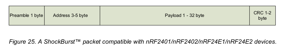
The S-band transmitter is based on a Nordic Semiconductor nRF24L01+ 2.4GHz FSK transceiver chip (see the datasheet here). The images are sent in 1Mbaud GFSK Shockburst packets. The structure of a Shockburst packet can be seen in the figure below, taken from the nRF24L01+ datasheet.

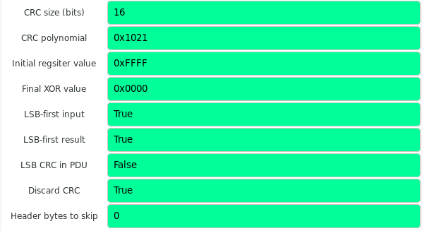
AMICal Sat uses the 5 byte address 0x7e7e7e7e7e, a 32 byte payload, and a 2 byte CRC. The CRC used by ShockBurst is the one called CRC_CCITT_FALSE in this online calculator, and covers both the address and the payload. The payload of each packet consists of a chunk counter, which is a 16-bit little endian integer, followed by a 30 byte chunk of the image file.

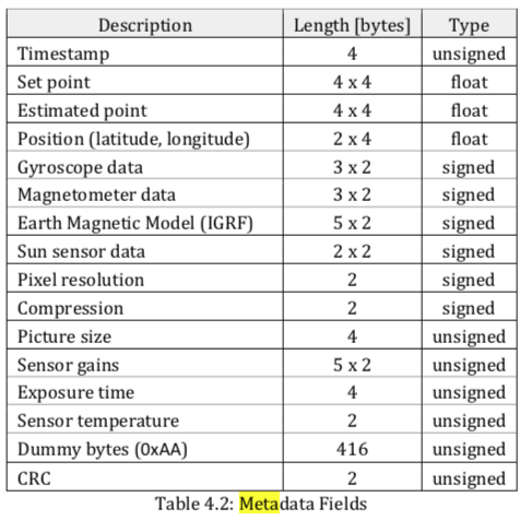
The image file has a 512 byte header followed by the image data. The header is described by the table below (all the fields are little endian).

The image data can be sent either uncompressed or compressed with fpaq0f2.

The main difficulty we’ve been facing is decoding all the packets without any bit errors. Even though Julien has made IQ recordings of the satellite in the lab, and the SNR is more or less good, it seems extremely difficult not to lose any packets due to bit errors.

In an attempt to reduced the errors, I have tried hard to design a reliable decoder in GNU Radio. The main ideas of this decoder are as follows. First, no clock recovery is done. This is acceptable, since the packets are rather short, and it increases reliability, as it eliminates the clock recovery loop as a possible point of failure. Four different clock phases are tried in parallel and packets decodes from all of them are stored for later processing.

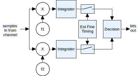
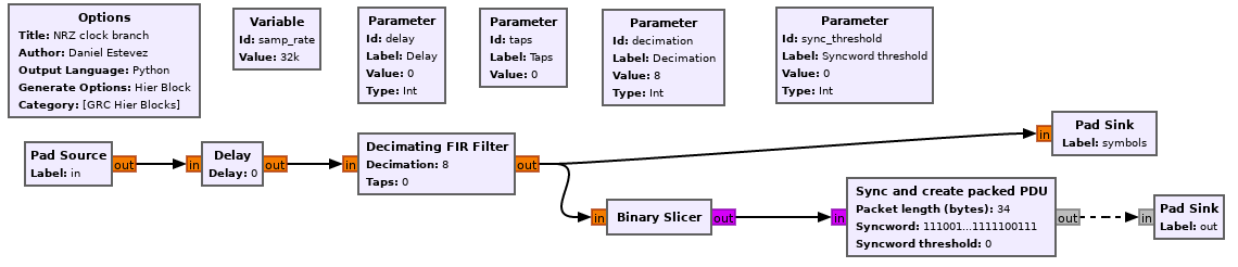
Second, there are two different decoding algorithms which are tried in parallel. The first one is an integrate and dump FSK demodulation algorithm. This is best explained by the diagram below, taken from this post in David Rowe VK5DGR’s blog.

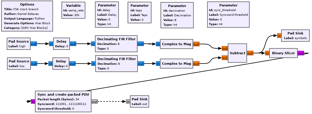
Essentially, each of the FSK tones is shifted to baseband, integrated coherently for a bit period, and then power is compared. This demodulator is implemented as a hierarchical flowgraph, which is instanced for each of the four clock phases. The flowgraph is shown in the figure below. The Sync and create packed PDU block from gr-satellites is used to detect the address and extract the payload and CRC as a PDU.

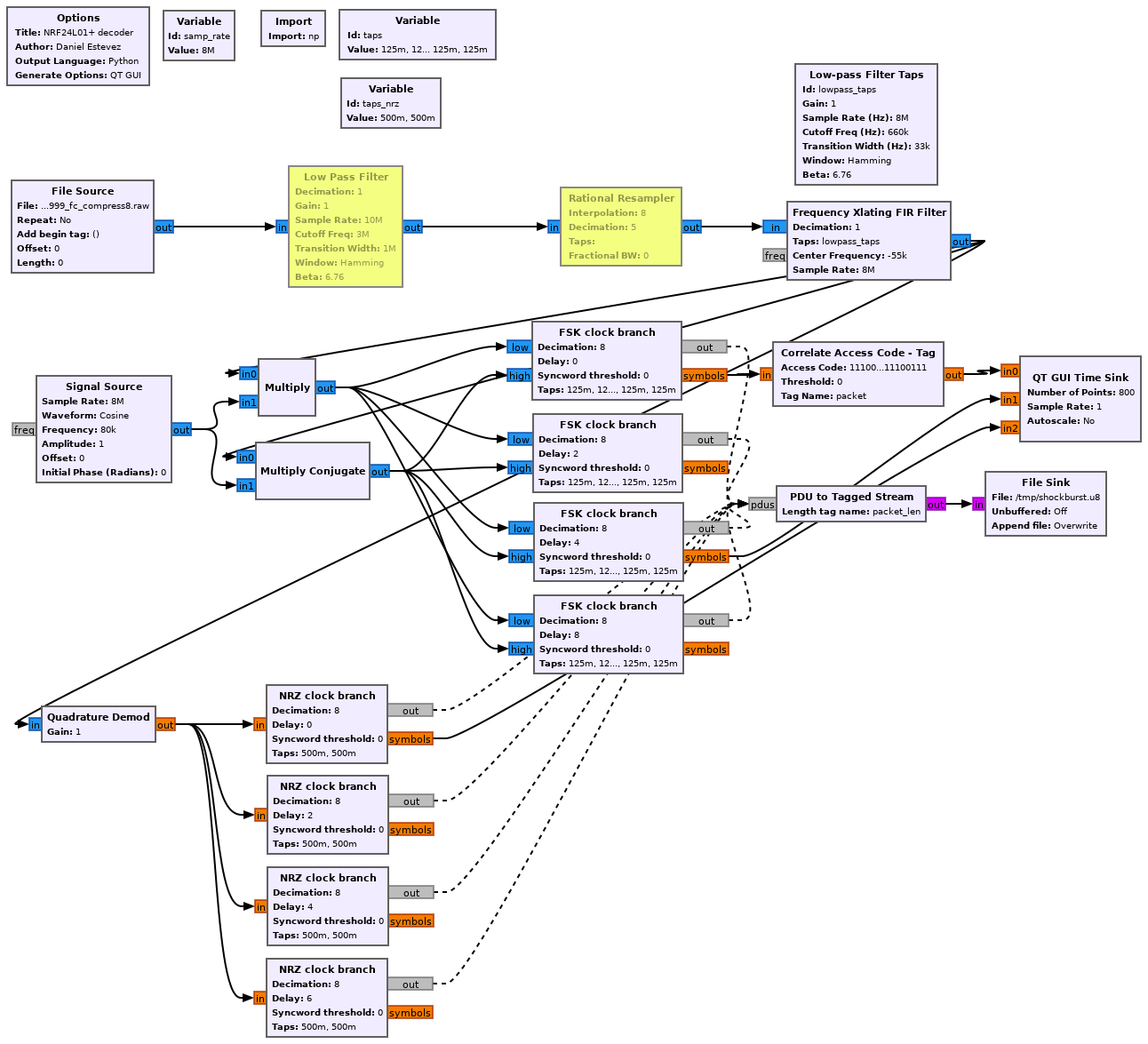
The second decoding algorithm is based on FM demodulation, followed by some filtering and bit slicing.

The full decoder can be seen in the figure below. There are four instances of the integrate and dump demodulator (called FSK clock branch) and four instances of the FM-based demodulator (called NRZ clock branch). Packets decoded from any of the branches are stored in a file for later processing.

The decoder flowgraph can be found in nrf24.grc.

After decoding, the frames are processed in this Jupyter notebook. It performs CRC checking, dropping all messages with invalid CRC. The remaining messages are grouped according to their chunk counter (first 2 bytes of the payload).

Ideally, we would expect that all the frames with the same chunk counter and correct CRC are equal (they are just the same frame decoded in parallel successfully by several of the eight demodulators). However, due to the short length of the CRC-16 code, we see many corrupted frames with valid CRC. To solve this problem, for each chunk counter value, a majority voting among the frames with that particular chunk counter value and correct CRC is done to try to select the correct frame. Often, the frame is decoded correctly by several of the eight demodulators, so this majority voting approach seems to work well to discard corrupted frames.

According to the result of the majority voting, the image file is reassembled using the chunk counter of each frame. Any missing frame leaves a gap of 30 bytes of zeros in the file.

Even after all this work, we haven’t managed to decode a transmission without any errors. The number of lost frames we get is quite low (on the order of 1%), but to recover compressed images we need perfect decoding, as any gaps in the file will make the decompression algorithm fail.

Image data

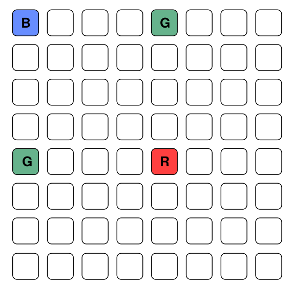
The image sensor used by AMICal Sat is an Onyx EV76C664 1280×1024 pixel sparse colour CMOS sensor. This means that whereas in most sensors the colour filter array has mainly coloured pixels, in this sensor most of the pixels are white, as shown by the figure below, taken from the datasheet.

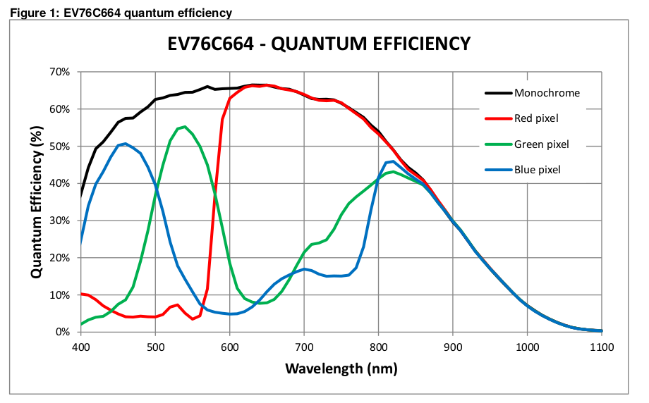
I don’t know much about image sensors, but the manufacturer claims that this gives the sensor better low-light performance, which seems reasonable and is very desirable for AMICal Sat use case. The figure below, also taken from the datasheet, helps illustrate the advantage of having many white pixels.

The sensor active area is 1408×1040 pixels, with a useful area of 1280×1024 pixels. The ADC has 14 bit depth, but often a lower depth, such as 12 or 10 bits is used.

The image sensor data can be sent as uncompressed raw ADC data or as raw ADC data compressed with fpaq0f2. We haven’t been able to decode a compressed image successfully, due to packet loss, but we have managed to put together some uncompressed images.

Raw ADC data is sent as little endian 16 bit integers scanning the full 1408×1040 sensor area. In these integers, only the 12 or 10 least significant bits are nonzero, depending on the image depth. Decoding of the raw data is done in this Jupyter notebook.

I don’t usually work with colour image data, so my background read on colour spaces and human colour perception has been quite interesting. To decode the image, first each of the R, G, B and Y (luminance, from white pixes) channels are extracted and interpolated to the full sensor size. Then, the chroma information in the RGB channels is converted to CbCr using the JPEG conversion. A translation is done in CbCr coordinates for white calibration (the appropriate translation has been determined experimentally with a calibration image). Finally, the CbCr information is taken together with the Y channel from white pixels and converted back to RGB. Note that this is a very naïve demosaicing algorithm and, specially given the low chroma resolution, gives suboptimal results.

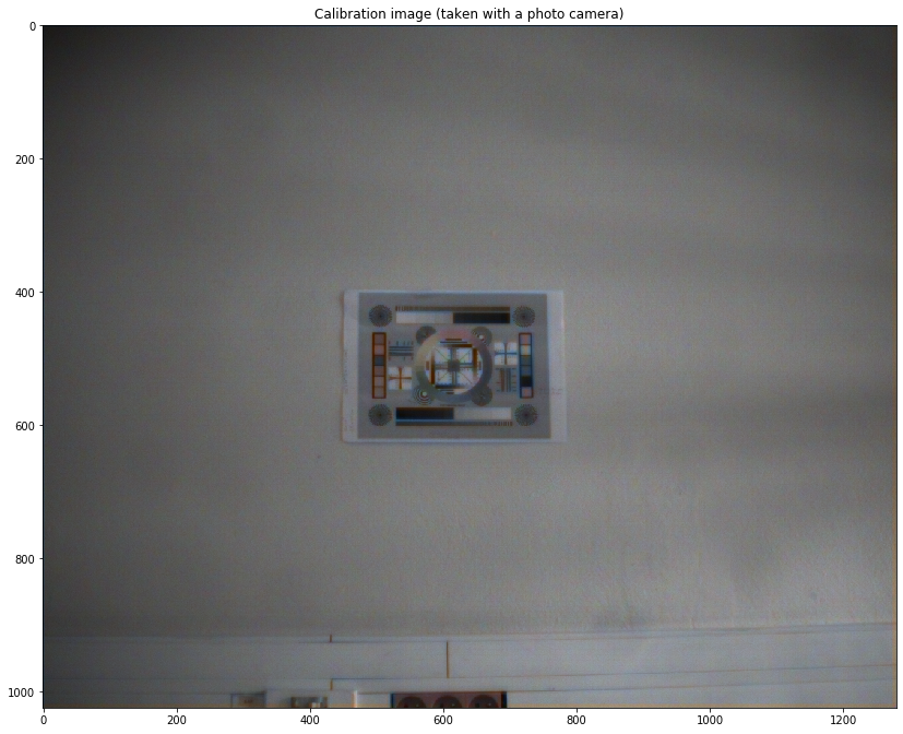
The first raw images I have worked with are a couple of calibration images taken in the lab. These are images of a calibration sheet taken at 12 and 10 bit depth. For some reason, the raw images have already been cropped to the 1280×1024 sensor useful size.

The figure below shows the calibration sheet photographed with a regular camera, for reference.

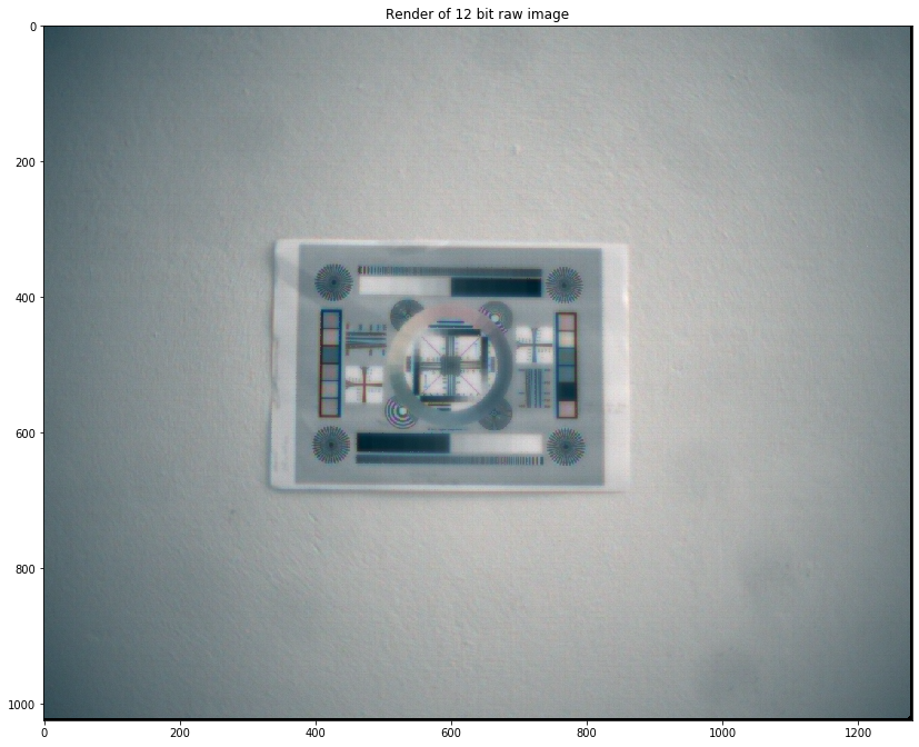
Below we show the image of the calibration sheet rendered from a 12 bit raw image taken with the AMICal Sat camera.

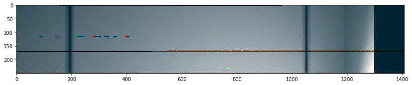
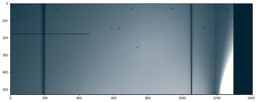
The two images below have been recovered from IQ recordings that Julien made of the S-band transmitter. The packet loss is apparent as black lines or very bright colours in some parts of the images. The data is 1408 columns wide, corresponding to the full sensor size. The useless sensor area can be seen as a dark stripe in the right side of the image. These images may not seem like much, but Julien tells me that they look like the corner in AMICal Sat’s clean room, so it seems all our software is working correctly.

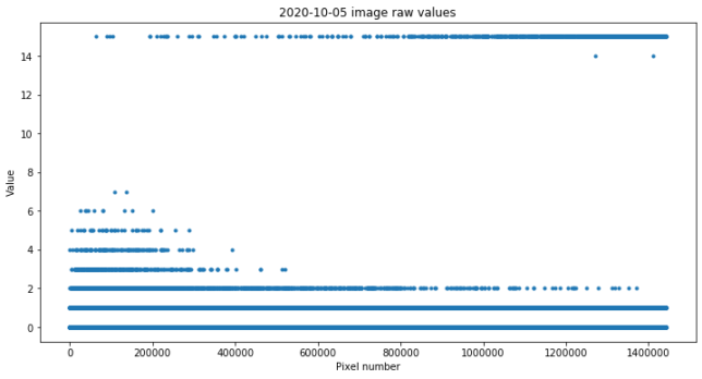
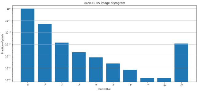
It is interesting to look at the useless sensor area on the right side of the image. For some reason, it is only 112 pixels wide, even though there are 128 useless pixels per row, according to the sensor datasheet. The figure below shows the histogram for the raw ADC values corresponding to these pixels. The data seems normally distributed with small variance, as if the ADC was held to a fixed voltage or left floating.

If we average the data by columns, it seems that there is a slight variation from left to right. Note that the variation is only around 3 ADC counts, while the standard deviation of the pixel values is 5.4 ADC counts, so averaging is needed to see this effect clearly. I don’t know anything about its cause.

BepiColombo is a joint mission between ESA and JAXA to send two scientific spacecraft to Mercury. The two spacecraft, the Mercury Planetary Orbiter, built by ESA, and the Mercury Magnetospheric Orbiter, built by JAXA, travel together, joined by the Mercury Transfer Module, which provides propulsion and support during cruise, and will separate upon arrival to Mercury. The mission was launched on October 2018 and will arrive to an orbit around Mercury on December 2025. The long cruise consists of one Earth flyby, two Venus flybys, and six Mercury flybys.

The Earth flyby will happen in a few days, on 2020-04-10, so currently BepiColombo is quickly approaching Earth at a speed of 4km/s. Yesterday, on 2020-04-04, the spacecraft was 2 million km away from Earth, which is close enough so that Amateur DSN stations can receive the data modulation sidebands. Paul Marsh M0EYT, Jean-Luc Milette and others have been posting their reception reports on Twitter.

Paul sent me a short recording he made on 2020-04-04 at 15:16 UTC at a frequency of 8420.535MHz, so that I could see if it was possible to decode the signal. I’ve successfully decoded the frames, with very few errors. This post is a summary of my decoding.

The X-band signal from BepiColombo is very similar to that of Solar Orbiter that I decoded a couple months ago, so I’ve been able to reuse most of the software. The signal is PCM/PM/Bi-φ modulated at approximately 700kbaud and uses an r=1/2 Turbo code with a block length of 8920 bits. Thus, the only difference between BepiColombo and Solar Orbiter is the baudrate (Solar Orbiter used approximately 555.5kbaud).

The SNR in this recording of BepiColombo is lower than in the Paul’s recording of Solar Orbiter, so my decoder didn’t work: the constellation locked, but it was too noisy for the Turbo decoder to correct all the bit errors. Therefore, I have tried an alternative decoding approach that seems to work better.

The decoder can be seen in the figure below. A PLL is used to track the residual carrier, phase demodulation is done, and the signal is resampled to 10 samples per symbol. After that, there is a FIR filter whose taps are a sequence of five -1’s and five +1’s. This should be thought as a matched filter to the Manchester pulse. At the appropriate sampling points, the taps of the filter are aligned with the Manchester clock and the filter wipes-off the Manchester modulation. After this we run clock recovery with the Gardner algorithm and then detect the 64bit ASM that marks the beginning of Turbo codewords.

I’m not completely sure that it’s impossible for this decoder approach to false-lock at 1/2-symbol offset from the correct symbol clock, but so far it seems to work well.

The GNU Radio decoder flowgraph can be found here. As in the case of the Solar Orbiter decoder, it uses gr-dslwp for Turbo decoding, so the flowgraph is for GNU Radio 3.7, as gr-dswlp hasn’t been ported to 3.8 so far. Note that Turbo decoding is very CPU intensive, so it would be really difficult to run the decoder in real time. When I run it on my i7-2620M laptop, the demodulator goes through the recording pretty fast, but the Turbo decoder stays running for many minutes until it finishes processing all the frames.

The decoder can be seen running in the figure below. The spectrum of the in-phase and quadrature branches of the PLL-locked signal is plotted, showing clearly the phase-modulated data sidebands in the quadrature component. There are many bit errors, but even so the Turbo decoder is capable of correcting all of them.

The analysis of the decoded frames can be seen in this Jupyter notebook and the file with the decoded frames is here in case anyone wants to have a more detailed look.

A total of 1808 frames were decoded from Paul’s 46.5 second recording. Only one of these has incorrect CRC. The frames are TM Space Data Link frames. According to the master channel frame count field, only 8 frames were lost in my decoding process.

Four different virtual channels are used to transmit the data. The relative usage of these can be seen below.

Virtual channel ID 0: 38 frames
Virtual channel ID 1: 99 frames
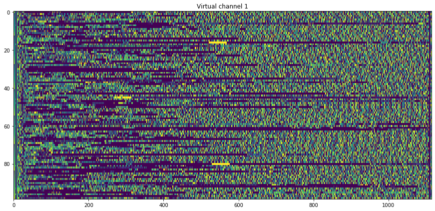
Virtual channel ID 2: 39 frames
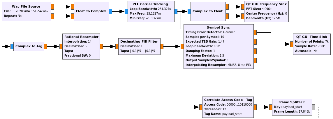
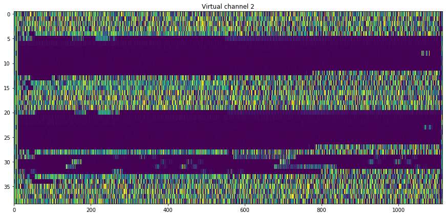
Virtual channel ID 7: 1631 frames

The contents of the virtual channels can be seen below. Each frame is plotted as one row of the graph, with colour-coded bytes. It can be seen that the data on each virtual channel is rather different. Virtual channel 2 is perhaps the most interesting, since it seems to have very long sequences of zeros. Virtual channel 7, where the bulk of the data is sent, shows some repetitive structure that doesn’t match the frame size.

I haven’t looked at the data in any more detail yet. What I’ve been curious about are the peaks that can be seen in the quadrature branch near the carrier. In fact, there are several peaks, as it can be seen in the figure below, which shows a close-in spectrum of the PLL-locked signal.

I’ve measured the frequency of these peaks to be 12490Hz, 22088Hz, 24981Hz, and 37417Hz, accurate to 1Hz or so. The last two are then 2nd and 3rd harmonics of 12490Hz. The 12490Hz and 22088Hz tones seem to be related by the fraction 4016/2271. This numerology is perhaps too much of a guess, but since 4016 and 2271 are coprime, it supports the idea that these are ranging tones. Indeed, 12490Hz/2271 is quite close to 5.5Hz (the error is 40ppm, which could be explained by Doppler and clock drift).

So my guess is that the 2271th and 4016th harmonics of a 5.5Hz clock are used for ranging. The ranging ambiguity is given by the 5.5Hz clock, and is approximately 5.5 millions of km. Regarding ranging performance, with a loop SNR of 20dB on the 22088Hz tone (which perhaps is not possible to achieve with this recording, but certainly it is not too far off), the tracking jitter of this tone would be 0.1rad RMS, which is equivalent to 216m, so this is actually not bad at all. However note that resolving the integer ambiguities would require averaging the phase jitter on the 22088Hz tone down to significantly less than 1mrad, so the SNR needed for unambiguous ranging is certainly much more than what is present in this recording.

When researching these tones I also measured the baudrate accurately by using cyclostationary analysis. It turns out that it is 699070.5 baud (accurate to around 1 baud), so I don’t think that the baudrate is related to the frequencies of these ranging tones.

The launch last Saturday of Crew Dragon Demo-2 undoubtedly was an important event in the history of American space exploration and human spaceflight. This was the first crewed launch from the United States in 9 years and the first crewed launch ever by a commercial provider. Amateur radio operators always follow this kind of events with their hobby, and in the hours and days following the launch, several Amateur operators have posted reception reports of the Crew Dragon C206 “Endeavour” signals.

It seems that the signal received by most people has been the one at 2216 MHz. Among these reports, I can mention the tweets by Scott Tilley VE7TIL (and this one), USA Satcom, Paul Marsh M0EYT. Paul also managed to receive a signal on 2272.5 MHz, which is not in the FFC filling, so this may or may not be from the Crew Dragon.

Scott has also shared with me an IQ recording of one of the passes, and as I showed on Twitter yesterday, I have been able to demodulate the data. This post is my analysis of the signal.

The recording that Scott sent me is 115 seconds long and was made on 2020-05-31 03:19:39 UTC, at a frequency of 2216 MHz using a sample rate of 4Msps. The recording has a size of 3.5GB. Interested people should get in touch with Scott to obtain a copy of the file. For convenience, I’m also hosting a one second snippet of this recording (selected from the portion where the signal was strongest). This snippet is only 31MB large and can be downloaded here. It should be more than enough for people interested in analysing the modulation and coding.

The material used in this post is in this Github repository. The data files are handled using git annex (see the README for instructions). The GNU Radio flowgraph crewdragon.grc uses some blocks from gr-satellites v3.0.0-rc1.

A first look at the modulation shows that it is FSK (most likely GFSK) with a baudrate of 2.35Mbaud and a deviation of approximately 800 kHz. I have made the demodulator shown below, which works by moving each of the two FSK tones down to baseband and comparing power.

The figure below shows the decoder running on the one second snippet linked above. Although there is lots of fading in the recording, the signal in this snippet is quite strong and there are very few bit errors. It is noteworthy the large number of spectral lines that are visible in the spectrum, as well as in the waterfalls of the tweets mentioned earlier.

This Jupyter notebook is used to look at the symbols produced by the demodulator and reverse-engineer the synchronization and coding. Since this is a spacecraft signal, it is quite possible that some form of the CCSDS protocols is used, and indeed correlating against the 0x1ACFFC1D CCSDS 32-bit ASM shows that this ASM appears in a regular fashion in the symbol stream.

The correlation peaks are spaced 2000 symbols. Not taking into account the 32 bit ASM, this suggests that frames of 1968 symbols are used. According to the TM Synchronization & Channel Coding CCSDS Blue Book, there are a number of coding schemes that use this 32 bit ASM: uncoded, convolutional, Reed-Solomon, concatenated, and some LDPC frames. However, the frame size doesn’t seem right for LDPC, and if a convolutional encoder was used, the ASM would be sent encoded, so we wouldn’t see it directly. This leaves us with uncoded and Reed-Solomon as the only choices (or it could be something else not in the Blue Book).

Collecting each of the frames as an array of 246 bytes and plotting them by rows, we get the figure below. We see that many frames have exactly the same pattern.

By looking at one of the frames with this pattern, we see that the pattern repeats every 255 bits and matches almost exactly the CCSDS scrambler sequence. This suggests that these are idle frames which are full of zeros almost completely. The fact that many frames have a repeating pattern of 255 bits explains the abundance of spectral lines, which should be spaced in integer multiples of 9215.7 Hz (for a clever solution to this, see my post about the BepiColombo idle frames).

By descrambling the frames, we see that only the first byte (which is 0xff) and the last 32 bytes are non-zero. This suggests that Reed-Solomon is used, and indeed a simple test with the Reed-Solomon decoder from gr-satellites shows that the frames can be decoded successfully with the CCSDS Reed-Solomon decoder using the dual basis.

Therefore, we conclude that the frames are completely standard CCSDS Reed-Solomon frames with a frame size of 214 bytes. The gr-satellites CCSDS Reed-Solomon Deframer can be used to perform ASM detection, descrambling and Reed-Solomon decoding. The resulting frames are written to a file, which is analysed in the same Jupyter notebook.

The figure below shows the successfully decoded 214 byte frames corresponding to the whole 115 second recording. Note that many frames, especially near the beginning and end of the recording, were not decoded due to the fading. In fact, there are some 130k frames in 115 seconds, while we only have nearly 60k correct frames.

The idle frames can be seen as dark lines, since all their contents, except for the first byte are zeros. It turns out that the first byte identifies the type of frame: 0xff for an idle frame, 0x00 for a non-idle frame. It is interesting to study the rate of idle frames, which shows the link usage. This can be seen in the figure below, where we can see some event that temporarily increases the datarate pushed through the link. Still, the link is nowhere near its maximum capacity (which is 243KiB/s, after discarding the overhead due to FEC and headers).

The second byte of non-idle frames contains a 7bit sequence counter (interestingly the most significant bit is always zero). We can use this counter to detect frame loss by looking at unexpected jumps in the counter (of course this has aliasing when many frames are lost and will ignore an integer multiple of 128 lost frames). The figure below shows that most of the time we manage to decode all the frames, but there are occasions when many frames are lost due to fading (note that this doesn’t take into account the moments when we don’t decode any frames at all).

The figure below shows all the non-idle frames that were correctly decoded. Except for the first two bytes, their contents seem completely random. It might happen that the data is encrypted or compressed, so without any knowledge of what kind of data is transmitted, it is not obvious how to proceed now.

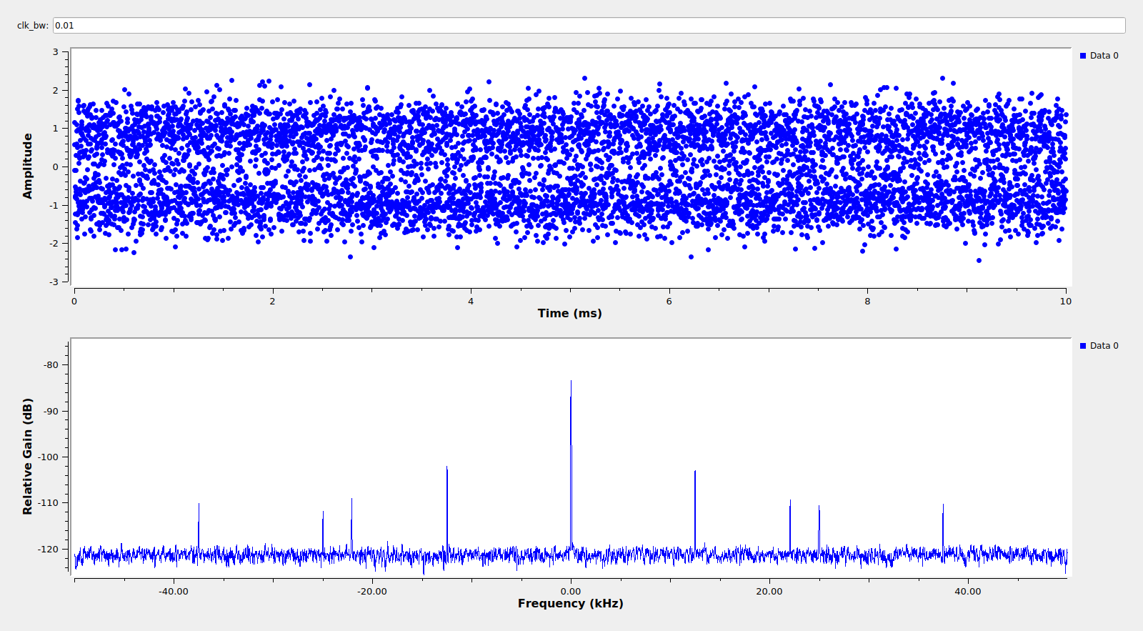
A few months ago I talked about BER simulations of the gr-satellites demodulators. In there, I showed the BER curves for the BPSK and FSK demodulators that are included in gr-satellites, and gave some explanation about why the current FSK demodulator is far from ideal. Yesterday I was generating again these BER plots to check that I hadn’t broken anything after some small improvements. I was surprised to find that the FSK BER curve I got was much worse than the one in the old post.

In the two figures below you can see the BER curve I got and the BER curve in my older post. The high SNR behaviour is nearly the same, but for low SNR the BER curve I got is much worse. The curve only starts “behaving well” at around 11dB Eb/N0, where the former curve started behaving well at maybe 7dB Eb/N0.

The reason for the change in regimes between a flat portion of the curve where the BER is 0.5, a transition region, and a portion where the demodulator “behaves well” is the clock recovery loop. When the SNR is below a certain threshold, the clock recovery loop doesn’t lock, so we are essentially decoding random garbage. In the transition region, the clock recovery loop barely locks, so it incurs a significant performance penalty. When the SNR is high enough, the clock recovery loop locks just fine and it doesn’t disturb the BER.

The threshold at which the clock recovery loop can lock is directly related to the clock bandwidth. A larger bandwidth will make locking faster, but will also bring the locking threshold up. The current default clock bandwidth in gr-satellites is 0.06. Repeating the simulation with a clock bandwidth of 0.02 I get the figure below, which is pretty close to the old figure.

Now, choosing the clock recovery bandwidth is a tradeoff between fast lock (which is needed to get packets with short preambles or unstable clocks) and low SNR performance. I have tried to optimize the default parameters for gr-satellites with many real world recordings, but in particular cases other parameter choices will work better.

I also find that the change in locking threshold from 7dB to 11dB Eb/N0 is perhaps not so significant as it might seem. Below 11dB Eb/N0 the BER is still pretty high even if the clock recovery has locked, so unless there is a good FEC cleaning all these bit errors, it is impossible to decode. Thus, we don’t really care whether the clock recovery can lock or not. In fact, many FSK Amateur satellites are still using AX.25 unfortunately. Since AX.25 has no FEC, anything below 13dB Eb/N0 or so is a no-go for these satellites.

As promised in this post, I will now speak about how to demodulate the Tianwen-1 telemetry signal. This post will deal with demodulation and FEC decoding. The structure of the frames will be explained in the next post. In this post I also give a fully working GNU Radio decoder that can store frames in the format used by the orbit state vector extraction Python script.

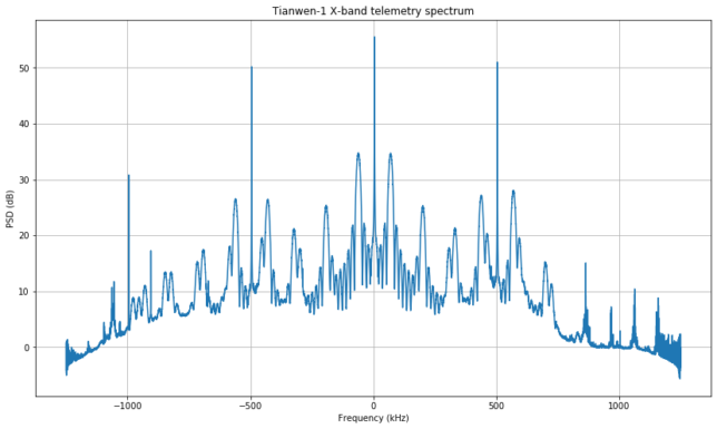
Tianwen-1 transmits an X-band telemetry signal at a frequency of 8431 MHz. As usual with deep space probes, the signal is phase modulated with residual carrier. Usually, the telemetry is transmitted at 16384 baud and modulated onto a 65536 Hz subcarrier. Following this terminology, it is a PCM/PSK/PM signal.

The figure below shows the GNU Radio decoder running on a recording made at Bochum earlier today. It displays the spectrum of signal, both before and after locking the residual carrier, so that signal quality and PLL lock can be assessed. It also shows the constellation symbols and filtered and unfiltered waveforms corresponding to the BPSK data subcarrier.

The figure below shows the full spectrum of the telemetry signal. This is taken from a recording made by AMSAT-DL with the 20m dish at Bochum observatory on 2020-07-26 07:47:20 UTC, after the spacecraft switched to its high gain antenna on 2020-07-26 00:30 UTC.

A thing to note here is that the data sidelobes only have odd harmonics. This means that the subcarrier is a square wave, because phase modulation with a sine wave produces both even and odd harmonics, while phase modulation with a square wave produces only odd harmonics.

Besides the central residual carrier and the data subcarriers at +/- 65.536 kHz, there are two CW subcarriers at +/- 500 kHz. Most likely these are used for ranging, as delta-DOR tones. Since everything is phase-modulated onto the same carrier, and phase modulation is inherently non-linear, everything intermodulates. Thus, we see the data subcarriers intermodulating with the CW subcarriers, and producing sidelobes at +/- 65.536 kHz from these (and also some odd harmonics).

In fact, with strong SNR, it is possible to lock the decoder onto one of the CW subcarriers and produce valid data from the intermodulation sidelobes. The figure below shows the decoder happily doing just that. Note the asymmetry of the spectrum, which is caused by the fact that the 7th and 9th harmonic of the data subcarrier also lie around here. This is more of a curiosity than something with a practical application.

The transmitter is also capable of high speed data. In fact, Ferruccio IW1DTU caught the probe transmitting what seemed like BPSK/NRZ (or maybe PCM/PM/NRZ with a weak residual carrier) on 2020-07-26 23:19 UTC. Unfortunately there is no recording of that event and we haven’t seen the spacecraft transmitting high speed data again.

Interestingly, Tianwen-1 has made an image of the Earth and Moon, and this appeared yesterday in the media. That high speed data event might have been used to transmit the image. The astute reader might be able to work out when the image was taken from the angular size of the Earth and the Moon, their angular separation in this image, and Tianwen-1’s trajectory. The media says that it was taken at 1.2 million km away, so according to my ephemerides table that would be around 2020-07-26 21:20 UTC.

The figure below shows the full decoder flowgraph, which can be downloaded here. Click on the figure to view it in full size.

The decoder can work with the recordings from Paul Marsh M0EYT, which use a sample rate of 249.995ksps, and with those made at Bochum, which use 2.5Msps, 625ksps or 312.5ksps (in all cases we decimate first to 312.5ksps). It can easily be adapted to use other sample rates.

To demodulate the signal we first use a PLL to lock the residual carrier. I’m using a loop bandwidth of 200Hz, and certainly it could be made smaller, but so far the SNR is strong enough for this high bandwidth and I don’t want to have problems with carrier dynamics due to the receiver clock or uncorrected Doppler.

After carrier recovery, we use the following method to demodulate the data subcarrier. First we take the imaginary part of the signal, since that is where most of the phase modulation power is. This has the effect of adding up the power in the two data sidebands to form a single BPSK signal at the subcarrier frequency.

An alternative idea to taking the imaginary part is to perform phase demodulation and use the complex argument instead, to try to use all the modulation power. I haven’t put much mathematical thought into this, but from some small experiments this works worse, at least for this phase deviation. Additionally, since phase demodulation is non-linear, the data subcarriers need to be bandpass filtered before taking the complex argument.

In any case, we end up with a real signal with a BPSK signal at the subcarrier frequency. We demodulate this as usual. We move it to baseband, obtaining an IQ signal again, then perform filtering (here I’m using a square-wave non-matched filter), clock recovery (done here with Gardner’s TED) and carrier recovery with a Costas loop. The Costas loop is actually locking to the subcarrier frequency, so its bandwidth can be kept rather small.

Note that the subcarrier frequency is actually four times the baudrate. This means that there are exactly four subcarrier cycles per symbol. This integer relationship is not a coincidence. Most likely the subcarrier and symbol clock are coherent, in the sense that if the symbols start at instants \(t = nT\) for \(n \in \mathbb{Z}\), then the subcarrier is \(\operatorname{sign}(\sin(8\pi t/T + \varphi))\) (or \(\sin ( 8 \pi t / T + \varphi ) \) for a sine wave subcarrier), where \(\varphi\) is typically chosen to be zero but can also be \(\pi/2\). This is the same as the BOC sine and BOC cosine waveforms in GNSS.

In practice, this means that the subcarrier and symbol clock are one and the same and could be recovered using the same loop, whose error can be fed from a weighted average of the TED and the Costas loop discriminator. I haven’t attempted to implement this technique.

After demodulation we perform frame synchronization and FEC decoding. The frames are CCSDS concatenated frames with a size of 220 bytes, as described in the TM Synchronization and Coding Blue Book. As pointed out by r00t, the conventional rather than the dual basis is used for the Reed-Solomon code, so this is somewhat non-compliant with CCSDS.

Though yesterday I commented about the fact that Beijing time is often used with Chinese spacecrafts, here I can’t offer much wisdom about the common use of Reed-Solomon by the Chinese. I can comment that the Amateur satellites made at Harbin Institute of Technology LilacSat-2 and BY70-1 use the conventional basis, and that the lunar satellites Longjiang-1/2, also made by Harbin, used the conventional basis for telecommand (Turbo codes were used for the downlink). In contrast, KS-1Q used the dual basis. Warmonkey, who worked in KS-1Q, made a very interesting comment back in the day about the computational advantage of implementing the conventional basis on a CPU and the dual basis on an FPGA.

The CCSDS concatenated deframer from gr-satellites is used to perform Viterbi decoding of the convolutional code, detect the 32 bit ASM and perform descrambling and Reed-Solomon decoding. We have a 180º phase ambiguity on the BPSK symbols. Even though the original PCM/PSK/PM signal doesn’t have any phase ambiguity, we’ve lost this with our Costas loop based subcarrier recovery. Another way of looking at this is that we haven’t used anywhere (and in fact we don’t know) the value of \(\varphi\) introduced above. Adding \(\pi\) to \(\varphi\) changes the phase of the BPSK symbols by 180º.

Therefore, two deframers are run in parallel: one on the stream of symbols, another on the stream of inverted symbols. Since there is also an ambiguity when pairing symbols at the input of the Viterbi decoder (this is handled inside the CCSDS concatenated deframer from gr-satellites), we have in fact four Viterbi decoders running in parallel.

After Reed-Solomon decoding is done, the 220 byte frames are stored into a file. This file can be read later with extract_state_vectors.py to print out the orbit state vectors that are sent in the telemetry.

I’ll close with two additional remarks. First, an anecdote and warning. When attempting to decode the signal, at first I assumed that the frame size was 223 bytes. This is a common frame size because it is the maximum allowed by a (255, 223) Reed-Solomon codeword. Due to the cyclic properties of Reed-Solomon codes, if we make a small mistake in the size, the decoder will still work.

For example, in this case the decoder takes three additional bytes of garbage (actually the first 3 bytes of the ASM of the next frame) after the real codeword, and provided there are not many byte errors in the real codeword it will just correct these three garbage bytes into the appropriate parity check bytes just as if they were byte errors (recall that such a Reed-Solomon code can correct up to 16 byte errors). The frame will be cropped to 223 bytes, leaving the first 3 parity check bytes at the end. These 3 bytes seem random, as if they were a CRC (and in fact I must recognize that I spent some time trying to see if they were a CRC-24).

So the lesson is to be careful about Reed-Solomon frame sizes and always check the number of byte errors corrected by the Reed-Solomon decoder. If this is never zero, suspect that maybe the frame size is wrong. Often there is no padding between frames, so the correct frame size can be observed by noting the distance between consecutive ASMs.

The final remark is about why a frame size of 220 bytes instead of 223 bytes. Well, there is a good reason. If we add to this the 32 Reed-Solomon parity check bytes and the 4 bytes of the ASM we end up with 256 bytes, which is a power of two, just like the baudrate. This means that, taking into account the convolutional encoding, a frame takes exactly 0.25 seconds to transmit. This is good because it allows a regular frame structure. For instance, the orbit state vectors can be sent every 32 seconds by sending one every 128 frames.

This is a post I had announced since I first described Tianwen-1’s modulation. Since we have very high SNR recordings of the Tianwen-1 low rate rate telemetry signal made with the 20m dish in Bochum observatory, it is interesting to make detailed measurements of the modulation parameters. In fact, there is something curious about the way the modulation is implemented in the spacecraft’s transmitter. This analysis will show it clearly, but I will reserve the details for later in the post.

Here I will be using a recording that already appeared in a previous post. It was made on 2020-07-26 07:47:20 UTC in Bochum shortly after the switch to the high gain antenna, so the SNR is fantastic. The recording was done at 2.5Msps, and the spectrum can be seen below. The asymmetry (especially around +1MHz) might be due to the receive chain.

The signal is residual carrier phase modulation, with 16348 baud BPSK data on a 65536Hz square wave subcarrier. There is also a 500kHz ranging tone.

The detailed measurement of the modulation is done with this GNU Radio flowgraph. Since the flowgraph is quite large, I will explain it by sections. The first section is just used to lock a PLL to the residual carrier. There is an AGC with a very long time constant, in order not to damp out any possible amplitude modulation in the signal. Then a PLL with a bandwidth of 500Hz is locked to the residual carrier. Here the large bandwidth is not a problem, since the carrier is very strong.

The GUI of the flowgraph is organized in tabs, since there are many GUI elements. The first tab is used to check correct carrier lock (note that only the central 250kHz of the modulation are shown in order to see the carrier better). We also show the constellation, which should look like an arc of circle symmetric about the point 1. However, we see that it is doesn’t have a perfect circular shape and it is somewhat asymmetric. This hints at some distortion in the form of amplitude modulation. As mentioned above, the distortion could be caused by the receiver.

The next part of the flowgraph gets the phase and amplitude of the phase-locked signal. The spectrum of these two real signals is plotted. We expect to see the modulating signals in the phase and no amplitude modulation. The data subcarrier and ranging tone are separated by means of a narrow bandpass that only lets through the 500kHz tone and its 2nd harmonic at 1MHz.

The output of this section can be seen below. In the spectrum of the phase modulation we see the BPSK data signal at 65536Hz and odd harmonics of the square wave subcarrier. We also see the 500kHz ranging tone and its 2nd harmonic some 22dB down. I don’t know why there is a 2nd harmonic, since there shouldn’t be regardless of whether the tone is a sine wave or a square wave. This might be caused by the signal distortion around +1MHz mentioned above. Most likely, in the undistorted signal the ranging tone is just a sine wave and there is no 2nd harmonic in the modulating signal (but the phase modulation will produce harmonics).

The amplitude modulation shows significant components at 500kHz and 1MHz, and a large number of spurs. The amplitude modulation will be investigated later.

The right hand side of the GUI shows the separated data and ranging signals in the time domain. The deviation of the data modulation (which will be measured later) is 0.725 radians. This is slightly less than \(\pi/4\), but it includes some possible losses in the measurement, so the real deviation might be \(\pi/4\). The deviation of the ranging tone is around 0.75, so again near \(\pi/4\). When both the data modulation and the ranging tone coincide, the total deviation is near \(\pi/2\), which agrees with the constellation shown above.

The next part of the flowgraph is used to investigate the relation between the BPSK symbol clock and the square wave subcarrier. To do so, we use the Symbol Sync block to lock to the subcarrier and output at 16 samples per symbol, so we get 32 samples per subcarrier cycle. An artificial subcarrier square wave is then generated at 32 samples per cycle and multiplied by the signal in order to wipe the subcarrier off and leave only the BPSK data modulation.

The figures below show the curiosity about the signal I mentioned at the start of this post. In this GUI tab we plot the following. In the upper left we show the data and subcarrier signal. There is no symbol shaping, so both the data and subcarrier are square waves. The subcarrier frequency is four times the baudrate, so there are four subcarrier cycles per symbol. This is what in the GNSS literature is called BOC(4) (GNSS isn’t directly related to deep-space communications but shares many similarities with these modulations). There are 8 subcarrier cycles plotted, so we have a total of two symbols. The red trace is a reference that shows what should the subcarrier look like in the absence of a data modulation.

The upper right plot is like the left one except that the waveform is multiplied by the reference subcarrier in order to remove the subcarrier and leave only the BPSK data modulation. Finally, the bottom plot shows the spectrum of the signal, from DC up to the 3rd subcarrier harmonic.

Now we note something interesting. If you look at the upper right plot, you’ll see that the BPSK symbol changes precisely at an edge of the reference subcarrier. This can also be seen in the Data + Subcarrier waveform in the upper left plot. There is a very short spike, but other than this the change in the BPSK symbol looks like a change in the phase of the subcarrier. We change from a subcarrier that has the same sign as the reference subcarrier to a subcarrier which has the opposite sign.

All the properties shown above happen because the subcarrier clock and the symbol clock are in-phase: the symbol changes happen at an edge of the subcarrier. This is called BOC-sine or BOCsin in the GNSS literature. However, this situation doesn’t maintain for long. Interestingly, it happens that in Tianwen-1 the subcarrier clock and symbol clock are generated from independent oscillators. These means that the frequency ratio is not exact and the clocks slide against each other.

In this particular recording, the period of the symbol clock is slightly larger than 4 subcarrier cycles. The effect in these plots is that the symbol transition keeps crawling to the right until eventually it happens in the middle of the subcarrier edges. This is shown below.

The subcarrier and symbol clocks are now in quadrature, and this modulation is called BOC-cosine or BOCcos in the GNSS literature. In the upper left plot we can see that the symbol change in the middle of the subcarrier edges produces one cycle of a square wave of frequency twice the subcarrier.

It is also interesting to compare the spectrums for the in-phase and the quadrature situations. When the subcarrier and symbol clock are in phase, the low frequency sidelobes between DC and the main lobe at 65536Hz have more power. When the subcarrier and symbol clock are in quadrature, the higher frequency sidelobes between the main lobe and the 3rd harmonic have more power.

As the subcarrier and symbol clocks keep sliding, the modulation keeps changing smoothly between the in-phase and quadrature configurations, exchanging power between the low frequency and higher frequency sidelobes. In this particular recording this happens every 1.4 seconds approximately, but we have seen other periods, since the clocks are free-running.

The video below shows the flowgraph GUI running so that you can watch how the symbol edges crawl slowly towards the right and how the power of the sidelobes alternates between the lower and higher frequency sidelobes. For this video, a throttle block was used to play the signal 10 times slower than real time.

The constant change between the in-phase and quadrature configurations produces a characteristic pattern in the signal when seen in a waterfall plot. Achim Vollhardt DH2VA called this “dancing”. See his tweet, which includes a short video. This effect also appears in the waterfall images posted by other Amateurs, such as Ferruccio IW1DTU.

The next and final section of the flowgraph performs clock recovery on the BPSK data signal (with the subcarrier already wiped off). Since the symbol pulse shaping is square, a square filter is used as a matched filter.

This is mainly used for two applications. First, to do a precise measurement of the amplitude of the symbols, which corresponds to the deviation of the data subcarrier, minus any small implementation losses. Second, for a measurement of the frequency difference between the symbol clock and the subcarrier clock. This section of the flowgraph works locked to the subcarrier clock, so any rate deviation of the recovered symbol clock from its nominal value indicates a frequency difference between the two clocks.

The GUI of this section of the flowgraph is shown here. We see that the symbols have very little noise due to the high SNR of the recording. The average amplitude of the symbols is around 0.725, as remarked above.

The precise measurement of the symbol clock fractional error is difficult, since this parameter probably varies with time. The value is around 3ppm. By doing the math, we see that with this frequency error, the configuration will change between in-phase and quadrature every 1.27 seconds.

Finally, there is a GUI tab that tries to show the amplitude modulation and relate it to the phase modulation of the 500kHz ranging tone. Both are passed through a narrow bandpass filter than only lets 500kHz and 1MHz through, since otherwise it is difficult to see any patterns in the time domain of the amplitude modulation. Since the signal distortion that causes amplitude modulation is probably at the receiving end, it is not easy to draw any definitive conclusions from this plot.

On 2020-09-04, China launched a “reusable experimental spacecraft” of which very little is publicly known. The most popular hypothesis is that this is a robotic spaceplane similar to the X-37B. The spacecraft spent two days in orbit and landed back at Earth, most likely near Lop Nur nuclear test site. Marco Langbroek has a nice post detailing all we know about the mission.

During the time it spent in orbit, the spacecraft released an object which has been catalogued as 2020-063G and is commonly known as “Object A”. On 2020-09-14, Dmitry Pashkov R4UAB detected an S-band signal coming from Object A at around 2280 MHz. This was verified later by Scott Tilley VE7TIL, who received a strong signal with lots of fading, suggesting that the object is tumbling. Marco also did some optical observations of the object.

Scott has sent me a recording of the S-band signal that he did on 2020-09-15 so that I can analyse it and we can learn more about this mysterious object. This post shows the results of my analysis.

The figure below shows the SNR of the signal recorded by Scott. We see that the signal appears from the noise shortly after 17:16 UTC and quickly rises in strength up to almost 15dB of (S+N)/N. There are many deep fades, and after a couple of minutes the signal disappears in the noise again.

The modulation of the signal is BPSK at 3069kbaud. I have used this GNU Radio flowgraph to demodulate the signal. The flowgraph has nothing special. It is just a simple BPSK demodulator that saves soft symbols and average power measurements into files.

The analysis of the symbols is done in this Jupyter notebook. Before we begin looking at them, let me remark something interesting about the baudrate. The number 3069 equals 3 times 1023, and 1023 kHz is the basic chip rate of GNSS signals. The use of this number started with GPS, which uses 1023 chip Gold codes, so as to give a 1ms code repetition interval. Modern GNSS signals are all based on multiples of 1023 kHz chip rates even if they no longer use PRN lengths of 1023 chips.

Therefore, the choice of a 3069 kbaud baurate might suggest that this is some kind of ranging signal, using a ranging code of length 1023 that is perhaps based on a 10 bit LFSR. However, this doesn’t seem to be the case.

The signal is clearly differentially encoded. The figure below shows the self correlation of a 2 second window of the symbol stream chosen where the SNR is strongest, so as to have few bit errors. There is almost no self-correlation.

However, if we perform differential decoding on the symbol stream, we see a strong self-correlation at lags multiples of 261888 symbols. This suggests a frame size of 261888.

Note that 261888 equals 256 times 1023, so again we have the number 1023 showing up. From here on, we will work with the differentially-decoded bitstream. If we arrange the bitstream in rows of 261888 bits, we get the figure below, which has been produced with 60 seconds worth of symbols.

We see that all the frames consist of almost the same pattern of 261888 bits. Occasionally there is a deep fade and clock recovery is lost, so we jump to another phase of the cyclic pattern.

Upon a closer look, we see that there are some bits that change. For instance, the figure below shows the first 256 bits of each 261888 bit frame, in a segment of data where there are no jumps due to clock recovery failure. We see that there are 6 bits that toggle occasionally. All the other bits maintain a constant value.

Moreover, it seems that there is a regular spacing between the bit positions that toggle. It is not difficult to identify the list of bit positions that toggle sometimes. I have studied this list to try to understand what is happening here.

In particular, I was trying to find a reasonable deinterleaving scheme that placed all the bits that toggle at the beginning of the frame. My idea was that maybe were are looking at frames that are scrambled and interleaved, and only the beginning of the frames contains valid data, while the rest is zeros. Thus, we would be looking mostly at the interleaved scrambler pattern, and some bits that correspond to valid data and are separated by the interleaver stride. However, the pattern doesn’t seem so simple, and I haven’t been able to come up with a good explanation.

In any case, it is true that the bit positions that toggle are separated by a rather regular spacing. To show this, we proceed as follows. We colour in yellow those positions that can toggle, and in purple the positions that never toggle, so we come up with a list of 261888 positions that are either yellow or purple. Next, we arrange that list in rows of 51 elements. The figure below shows the first 50 of those rows. The pattern continues “snaking” towards the right (and looping back to zero) on the following rows.

We see that there are a few rows where a single yellow square appears in the same position. Then a new yellow square appears in the following position, and this state with two yellow squares per row persists for only one or two rows. In the next row the left yellow square disappears, so the pattern has moved one position to the right.

Alternatively, we can write our list of positions as a set of indices and show the quotient and remainder of these indices when divided by 51. Note that this is essentially the same as the figure above. The beginning of this list of quotient and remainder pairs looks like this (the line jumps have been added for clarity):

(0, 39),   (1, 39),  (2, 39),
(2, 40),   (3, 40),  (4, 40),  (5, 40),  (6, 40),  (7, 40),  (8, 40),  (9, 40),
(9, 41),  (10, 41), (11, 41), (12, 41), (13, 41), (14, 41), (15, 41),
(15, 42), (16, 42), (17, 42), (18, 42), (19, 42), (20, 42), (21, 42), (22, 42),
(22, 43), (23, 43), (24, 43), (25, 43), (26, 43), (27, 43), (28, 43),
(28, 44), (29, 43),
(29, 44), (30, 44), (31, 44), (32, 44), (33, 44), (34, 44), (35, 44),
(35, 45), (36, 44), 
(36, 45), (37, 45), (38, 45), (39, 45), (40, 45), (41, 45), (42, 45),
(42, 46), (43, 46), (44, 46), (45, 46), (46, 46), (47, 46), (48, 46), 
(48, 47), (49, 46),
(49, 47), (50, 47), (51, 47), (52, 47), (53, 47), (54, 47), (55, 47),
(55, 48), (56, 48), (57, 48), (58, 48), (59, 48), (60, 48), (61, 48), (62, 48),
(62, 49), (63, 49), (64, 49), (65, 49), (66, 49), (67, 49), (68, 49), (69, 49),
(69, 50), (70, 50), (71, 50), (72, 50), (73, 50), (74, 50), (75, 50),
(76, 0),   (77, 0),  (78, 0),  (79, 0),  (80, 0),  (81, 0),  (82, 0),  (83, 0),
(83, 1),   (84, 1), ....

I have no clue what we’re looking at here. The pattern shown in the figure above can be described by saying that it’s a series of vertical “sticks” that move to the right and overlap at their endpoints. However, the heights of these sticks vary. There are sticks of lengths 7, 8 and 9. The overlap also changes between one and two rows. So there is certainly a lot of regularity, but it isn’t a totally trivial pattern, such as the one produced by a matrix interleaver. It may happen that we’re missing to identify some bits that may toggle between different frames, but don’t.

I think that the fact that we have these toggling bits discards all ideas about a ranging code or a CDMA system. It wouldn’t make sense to toggle a few individual chips in such a system. It would also be quite strange to use differential encoding with a ranging code or CDMA signal.

An important remark is that these bits that toggle are not caused by symbol errors. Since we are doing differential decoding, a symbol error would cause two adjacent bits to toggle, which doesn’t happen here.

One thing is clear: the signal doesn’t have much data in it, as most of the bits show the same repeating pattern.

Here I end my analysis, since by now I don’t have any clever ideas to explain the structure we see in the bitstream. The original IQ file and the stream of soft symbols are too large to share conveniently, but in the Github repository I have included a file with the 60 seconds worth of differentially decoded symbols. This file has a size of only 22MB and it should be sufficient for anyone that wants to continue the analysis where I left it. The file can be downloaded with git-annex as indicated in the README.

Back in March, I was helping Julien Nicolas F4HVX to test the S-band image transmitter of AMICal Sat before launch. In my post back then, I explained that AMICal Sat uses a Nordic Semiconductor nRF24L01+ 2.4GHz FSK transceiver chip to transmit Shockburst packets at 1Mbaud. I also explained how the Onyx EV76C664 CMOS image sensor works and how to process raw images.

AMICal Sat was finally launched on 2020-09-03, and since them the satellite team has been busy trying to downlink some images, both using the UHF transmitter (which uses the same protocol as Światowid) and the S-band transmitter. This has proven a bit difficult because the ADCS of the satellite is not working, and the downlink protocols are not very robust.

Julien has been sending me recordings done by their groundstation in Russia with the hope that we could be able to decode some of the data. Before several failed attempts where we were hardly able to decode a few packets, we got a particularly good S-band recording done on 2020-10-05. Using that recording, I have been able to decode a full image.

The recording is a 7.5Msps IQ recording that lasts for about 65 seconds. The frequencies in the recording are inverted, as one can check by examining the AMICal Sat Shockburst frames and noting that the characteristic 0xe7e7e7e7e7 address in inverted. Therefore, it is necessary to invert the frequencies by taking the complex conjugate or swapping I and Q before continuing. I don’t know the centre frequency of the recording, but the AMICal Sat signal can be found at -1.55MHz in the original recording.

Below we can see one of the Shockburst packets from the recording being FM demodulated in inspectrum. Note that there is a huge frequency drift at the beginning of the packet. Luckily, by the time that the 0xe7e7e7e7e address starts (which is what I use for frame synchronization), the frequency is already settling.

In hindsight, this frequency drift problem was already present in the pre-flight recordings we used in March. This, together with the lack of a moderately long preamble in Shockburst packets is what made me spend some time tuning an FSK demodulator for these short bursts.

The decoder that I have used is basically the same GNU Radio flowgraph to decode Shockburst packets that I used in March. It can be obtained here. The flowgraph saves all the frames that have a 0xe7e7e7e7e7 address with no bit errors into a file, regardless of whether the CRC is correct. Several copies of each frame are usually stored in the file, since there are multiple decoders in parallel trying different clock phases.

The Shockburst packets are then analyzed in this Jupyter notebook, which I have adapted from my work in March. First we filter out the frames having incorrect CRC-16. The first 2 bytes of each packet (after the address) contain a frame counter that increases starting from zero to indicate which chunk of the file is being transmitted.

The value of this field is shown in the figure below. The large spikes correspond to packets whose frame count field contains 0x5555. These packets are special and seem to indicate that a file downlink is starting. We see that after these packets the frame counter starts from zero and keeps increasing until the whole file is transmitted, and then gets back to zero as a new transmission starts.

There are five transmissions in total, which are separated by a gap of several seconds with no signal. The file sent in each of the transmissions is actually the same one. By sending the same file multiple times, the chances of successfully receiving all the frames are maximized.

The special packets that contain 0x5555 in their frame count field are all the same and contain the following payload (not including the CRC-16):

55555555555555555555555555555555555555555555555555555555a0760000

They are very easy to see in the spectrum, due to the long string of 0x55 bytes and the lack of a scrambler. Note that we don’t have special packets between the first and second transmission. This is just because we haven’t been able to decode any of these special packets correctly, as they are clearly present in the recording.

The figure below shows the start of the transmission (WiFi interference included). We see 17 of these special packets, which show a strong carrier, and then the regular packets containing the file chunks.

I have put together some code that assembles a file by using the frame count and detects the number of missing packets that were skipped. When we treat each transmission individually, we obtain the following:

Skipped 15 / 948 frames
Skipped 30 / 948 frames
Skipped 25 / 948 frames
Skipped 26 / 948 frames
Skipped 37 / 948 frames

We see that there is a frame loss of around 2.5%. However, when we take into account that these are five repetitions of the same file, we can put together the whole file without any missing frames. The file has 28470 bytes and can be downloaded here.

As I explained in my post in March, the start of the file has a 512 byte header with metadata. I have made a Jupyter notebook to parse the metadata according to the table I showed in that post. However, I have needed to make some minor modifications to the fields by adding a couple of padding fields that were not present in the table. Julien has helped me with this by showing me the metadata values obtained with the software that the team is using. The padding fields are quite easy to spot because they contain 0xaa bytes. The contents of the metadata header are as follows:

Container: 
    timestamp = 1601326224
    set_point = ListContainer: 
        -3.0316488252093987e-13
        -3.0316488252093987e-13
        -3.0316488252093987e-13
        -3.0316488252093987e-13
    estimated_point = ListContainer: 
        -3.0316488252093987e-13
        -3.0316488252093987e-13
        -3.0316488252093987e-13
        -3.0316488252093987e-13
    lat_lon = ListContainer: 
        -3.0316488252093987e-13
        -3.0316488252093987e-13
    gyroscope = ListContainer: 
        43690
        43690
        43690
    magnetometer = ListContainer: 
        43690
        43690
        43690
    earth_magnetic_model = ListContainer: 
        43690
        43690
        43690
        43690
        43690
    sun_sensor = ListContainer: 
        43690
        43690
    pixel_resolution = 8
    compression = 1
    dummy0 = b'\xaa\xaa' (total 2)
    picture_size = 27934
    sensor_gains = ListContainer: 
        64
        32896
        32896
        0
        1920
    dummy1 = b'\xaa\xaa' (total 2)
    exposure_time = 1000000
    sensor_temperature = 223
    dummy = b'\xaa\xaa\xaa\xaa\xaa\xaa\xaa\xaa\xaa\xaa\xaa\xaa\xaa\xaa\xaa\xaa'... (truncated, total 412)
    crc = 10481

The timestamp seems correct and is the UNIX timestamp for 2020-09-28 20:50:25, which I guess makes sense. Most of the fields don’t contain valid data, presumably because the ADCS system is not working.

The rest of the file contains a raw image compressed with the fpaq0f2 algorithm. The fpaq0f2 software is a simple C++ program. The file can be decompressed like so:

$ tail -c +513 compressed_image_with_header > compressed_image_no_header
$ g++ -o fpaq0f2 fpaq0f2.c
$ ./fpaq0f2 d compressed_image_no_header raw_image
compressed_image_no_header (27937 bytes) -> raw_image (1441792 bytes) in 0.46 s.

The raw image we obtain is a 704×1024 pixel 12 bit image. Each pixel value is stored as a little-endian uint16_t, and the sparse colour pixel arrangement of the sensor follows what I described in my post from March. It is interesting that the horizontal resolution has been decimated by 2. The full images from the sensor are 1408×1024, of which only the leftmost 1280 columns are usable.

After running the image through my code that converts it to an RGB image, we obtain the following.

There is not much to see here. The band on the right is the unusable area of the image, and looks the same as in those images taken in the lab in March, but with many hot pixels, especially in the bottom. The usable area of the image is very dark, but there are a few pixels that are brighter than the rest. We can exaggerate this by pretending that the image is 9 bits depth instead of 12, so anything having a value of more than 1/8th full scale will saturate.

Note that colour pixels (especially blue and red) have an effect over a relatively large area of the image and show up as a small blob rather than a dot. This is just because the resolution of the blue and red pixels is 1/8th of the total resolution (in both the vertical and horizontal directions), so the value of these pixels is assigned to the small area of 8×8 pixels surrounding them (I’m actually oversimplifying the image processing algorithm to explain this).

It is also interesting to look at the raw pixel values, shown below.

Some of the values are quite near the full scale of 4095. I think these correspond to hot pixels that are either dead or perhaps affected by radiation when the image was taken. The other values seem to cluster around multiples of 256, which is quite surprising. I don’t know what could cause this.

We can study this in more detail in the following histogram, which shows the relative proportion in which the different pixel values appear. Note that the vertical scale is logarithmic (in fact most of the pixels have the value 0, so we would see nothing in a linear scale), and that the horizontal axis has jumps (we jump from 15 to 256, for instance). These are all the pixel values that appear in the image. It is surprising that there are relatively few, rather than having values spread over a continuum.

The image processing code can be found in this Jupyter notebook. Currently the satellite team is studying this image in more detail to see what else can be learned from it. Best of luck to the AMICal Sat team with their mission.

Update 2020-10-12: Julien has made me notice that the raw image is actually 8 bits depth stored as uint8_t, rather than 12 bits stored as uint16_t. This explains why I thought that the horizontal resolution was 704 pixels, half the normal of 1408 pixels. It also explains the clustering of values around multiples of 256. In fact, the most-significant-byte of each uint16_t was actually the value of another pixel.

With this in mind, I have updated the notebook. The image is now as follows.

As we can see in the histogram below, all the pixel values are below 16, from a possible maximum of 255. In fact, most “hot pixels” are 15, while it would make sense for them to be 255.

I’m guessing that maybe the conversion from 12 bits to 8 bits is not correctly implemented, and leaves only 4 valid bits. Rescaling the values as if it was a 4 bit image, we obtain the image below. Now the band on the right is visible and has the same aspect as in the pre-flight images done in the lab.

In fact, most of the pixel values in this band on the right are 1. On the 12 bit images done in the lab the values in this band were around 200. Therefore, after a division by 16 to pass to 8 bits, we would expect values around 12. However, if instead we do a rounded division by 256, then we get 1. This supports my idea that the image has been inadvertently left with only 4 bits of depth.

NEXUS, also called FO-99, is a Japanese Amateur satellite built by Nihon University and JAMSAT. It was launched on January 2019, and one of its interesting features is a π/4-DQPSK high-speed transmitter for the 435 MHz Amateur satellite band.

I was always interested in implementing a decoder for this satellite, due to its unusual modulation, but the technical information that is publicly available is scarce, so I never set to do it. A few days ago, Andrei Kopanchuk UZ7HO asked me a question about the Reed-Solomon code used in this satellite. He was working on a decoder for this satellite, and had some extra documentation. This renewed my interest in building a decoder for this satellite.

With some help from Andy regarding the symbol mapping for the π/4-DQPSK constellation, I have made a decoder GNU Radio flowgraph that I have added to gr-satellites.

The modulation used by NEXUS is actually listed as π/4-QPSK 38k4 in several sites, such as in the satellite operations schedule. However, to be more precise, the modulation is 19.2 kbaud π/4-DQPSK. This means that each pair of bits is encoded as the phase shift between one symbol and the next one. There are four possible phase shifts: \(\pi/4\), \(3\pi/4\), \(5\pi/4\), and \(7\pi/4\).

Thus, if the constellation is rotated appropriately, the constellation symbols are \(1\), \(i\), \(-1\), \(-i\) for even symbols, and \((1+i)/\sqrt{2}\), \((-1+i)/\sqrt{2}\), \((-1-i)/\sqrt{2}\), \((1-i)/\sqrt{2}\) for odd symbols. These are two QPSK constellations staggered by a 45 degree rotation.

The symbol mapping used by NEXUS to transform the phase differences between adjacent symbols into dibits is shown in the table below, together with the more usual QPSK symbol mapping that assigns to the constellation symbols \(z = \pm 1 \pm i\) the dibit given by \((\operatorname{Re}(z)+1)/2\), \((\operatorname{Im}(z)+1)/2\) (here the function \(t \mapsto (t+1)/2\) represents justs a bipolar to unipolar transformation, so that the symbol mapping accounts essentially to taking the real and imaginary parts of the symbol, which is very useful for decoding).

Comparing the NEXUS symbol mapping with the usual QPSK mapping, we see that we can convert between them by inverting the bits and swapping I and Q, so this gives an effective way of decoding the NEXUS symbol mapping. However, the NEXUS symbol mapping can be constructed in a more natural way by taking the usual order of the 2-bit Gray code, indexed by the phase differences in increasing order.

The baudrate (symbol rate) for the NEXUS signal is 19.2 kbaud. Probably the signal is listed as 38k4 because the bitrate (not taking FEC into account) is 38.4 kbit/s.

The frames transmitted in this signal are standard CCSDS Reed-Solomon frames with a frame size of 223 bytes (not counting the 32 Reed-Solomon parity check bytes). The dual basis is used for the Reed-Solomon code.

The payload of each Reed-Solomon codeword contains a single AX.25 frame, using some sort of HDLC encoding. The best way to describe this encoding is that if we take the payload and invert the bit ordering in each of the bytes (i.e., if we replace \(b_7b_6\ldots b_1b_0\) by \(b_0b_1\ldots b_6b_7\)), then we obtain a perfectly compliant AX.25 frame using HDLC. Bit stuffing, the LSB byte ordering of AX.25, and the CRC-16 CCITT are used. The payload starts by a single 0x7e flag, and after the AX.25 frame, 0x7e flags are repeated until the end of the payload. These final 0x7e flags may or may not be byte-aligned depending on the amount of bit stuffing. This is represented by the image below, which Andy has shared. Note that the zero padding field should actually be 0x7e padding.

This frame structure is quite interesting, because it resembles FX.25 in that an AX.25 frame is wrapped by an outer FEC layer. FX.25 is designed to be backwards compatible with AX.25, since an AX.25 receiver will just ignore the wrapping. However, the NEXUS framing is not AX.25-compatible, because of the CCSDS synchronous scrambler and also because the bit ordering in each byte needs to be inverted.

I am curious about why this frame structure was used, since it doesn’t give backwards compatibility with AX.25 receivers (and in any case, there are no 19k2 π/4-DQPSK AX.25 modems that I know of, so backwards compatibility is not very useful). If backwards compatibility is not desired, then it seems much more simple to include the AX.25 frame directly into the Reed-Solomon codeword payload, without using any of the HDLC features (though some way to mark the frame end or length would be needed).

The GNU Radio decoder flowgraph is shown in the figure below. The recording I’ve used has been provided by Andy and can be downloaded here. It uses 96ksps real sampling and the signal is centred at about 18750 Hz.

A Frequency Xlating FIR Filter is used to move the signal to IQ baseband at 48ksps. Then there is an AGC and the Symbol Sync block, that performs RRC matched filtering and symbol clock recovery.

Each symbol is multiplied by the complex conjugate of the preceding symbol in order to get a constellation that gives the phase difference between adjacent symbols. This constellation is decoded to dibits by using the relation with usual QPSK constellation explained above.

Then the gr-satellites CCSDS Reed-Solomon deframer is used to synchronize to the CCSDS frames, descramble and decode the Reed-Solomon code. The bytes in the payload are reflected to invert the bit ordering and then sent into the HDLC deframer, which checks the CRC-16 and outputs the AX.25 frames.

Note that this decoder uses non-coherent demodulation of the differential constellation. Another approach would be to use coherent decoding by including a Costas loop. One way to do so would be to contra-rotate every other symbol by 45 degrees at the output of the Symbol Sync block, in order to compensate for the constellation staggering. Then a regular QPSK Costas loop can be used. At the output of the Costas loop, the 45 degree contra-rotation can be undone. Then the decoding can proceed as in the non-coherent case, by multiplying each symbol with the complex conjugate of the previous one.

One of the interesting Amateur cubesats in yesterday’s SpaceX Transporter-1 launch from Cape Canaveral is IDEASSat, a 3U cubesat from the National Central University of the Republic of China (Taiwan) designed to study ionospheric plasma. Jan van Gils PE0SAT drew my attention to this satellite as he was trying to see if it was possible to decode it with any of the decoders existing in gr-satellites. Mike Rupprecht DK3WN also helped with a good recording, much cleaner than the SatNOGS recording that Jan was using.

Presumably this satellite uses “AX25, 9k6, GMSK”, as listed at the bottom of this page from Taiwan’s National Space Organization, and also in this research paper. However, this is not true. It’s simple to check that the usual 9k6 FSK AX.25 decoders aren’t able to decode this signal, and a look at the FSK symbols shows that there is no scrambler (9k6 AX.25 uses the G3RUH scrambler) and that the symbol sequence doesn’t have much to do with AX.25.

After some reverse-enginnering, yesterday I figured out how the coding used by IDEASSat worked, and today I added a decoder to gr-satellites to help Mike investigate what kind of telemetry the packets contain. The protocol is not very good, so I think it’s interesting to document it in detail, as some sort of lessons learned. In this post I’ll do so. As it turns out, the protocol has some elements that loosely resemble AX.25, so I’m left wondering whether this is some unsuccessful attempt at implementing standard AX.25 (we’ve already seen very weird attempts, such as ESEO).

An excerpt of the recording that Mike sent me can be found as ideassat.wav in my satellite-recordings repo. From the recording, which is already FM-demodulated, it is clear that the modulation is 9k6 FSK.

The first thing that shocked me when looking at Mike’s recording is that there doesn’t seem to be any preamble. The packet starts directly with the data, as shown here. This is very bad, because closed-loop clock recovery algorithms need a preamble to lock to the symbol clock.

There is another bad thing about the FSK burst. If we look at the full burst, we see that before and after the burst there is a part that starts negative and slowly decays exponentially to zero.

This is caused by the fact that the FSK low tone is held for some 100ms before and after the FSK burst. Doing this at the beginning of the burst is a bad idea. Most FSK demodulators are AC coupled. Even the digital ones, as they use this to correct for frequency errors. So if one of the FSK tones is held for a significant amount of time, AC coupling will drive this tone to zero (just as we see with Mike’s recording). Thus, when the FSK burst starts, it will do so with a large DC offset, as we can see in the first figure.

In any case, all these problems can be sorted out (at least for manual inspection) by using a DC block in GNU Radio to correct for the DC offset at the beginning of the burst and Mike Ossman’s whole packet clock recovery script to extract all the symbols in the burst regardless of the lack of preamble.

After looking at the symbols for a while with NumPy, I realized that they were NRZ-I encoded UART-like data. By NRZ-I I mean the usual differential encoding from AX.25, where a 0 is encoded as a symbol change and a 1 is encoded as no symbol change. I say UART-like because it is exactly like 8-bit UART with one stop bit and no parity (1N8 for short) except for the fact that bytes are transmitted most-significant-bit first, whereas most UART transmit bytes in least-significant-bit first ordering.

The clues that lead me to this conclusion are the following:

• Differential decoding yields a richer autocorrelation than if we don’t do differential decoding; it’s always handy to see how differential decoding changes the autocorrelation
• After differential decoding, the autocorrelation showed peaks every 10 bits, and much larger peaks every 400 bits (which I’ll explain later)
• Arranging the symbols in 10 bit segments, there were two adjacent bits that had constant and opposite values; these strongly suggest the stop and start bits of UART
• The fact that the start bit of UART must be zero and the stop bit must be one indicates NRZ-I rather than plain differential decoding (the two are related by a bitwise inversion)
• When interpreting the UART bytes as most-significant-bit first, I got ASCII data

When decoded as NRZ-I 1N8 MSB UART, I got the following data in hex. The line breaks are mine for clarity and I’ve corrected a few obvious bit errors at the beginning by hand.

7e424e3043552030424e3049444130f000f4b2420741c3d042787fffdf021520000000000101007e
7e424e3043552030424e3049444130f001000101030401ffff07800720071807800728071800007e
7e424e3043552030424e3049444130f0020300670b0b0000000000000000089b04810cb8044b0d7e
7e424e3043552030424e3049444130f003b7035a032101a80cd802800cb80058176800080778007e
7e424e3043552030424e3049444130f00408071800080710fbf81fe000181fe001802f100000007e
7e424e3043552030424e3049444130f005000000000004f800004230424d46554e0000000000007e
7e424e3043552030424e3049444130f0060000000000000000000000000000000000000e6a00ba7e
7e424e3043552030424e3049444130f00707d0ff230c76f483d9cef5c2d4f0ad3047025d8100007e
7e424e3043552030424e3049444130f008271000002b14f81cf51afd00000000000000000000007e
7e424e3043552030424e3049444130f000f4b2420741c3d042787fffdf021520000000000101007e
7e424e3043552030424e3049444130f001000101030401ffff07800720071807800728071800007e
7e424e3043552030424e3049444130f0020300670b0b0000000000000000089b04810cb8044b0d7e
7e424e3043552030424e3049444130f003b7035a032101a80cd802800cb80058176800080778007e
7e424e3043552030424e3049444130f00408071800080710fbf81fe000181fe001802f100000007e
7e424e3043552030424e3049444130f005000000000004f800004230424d46554e0000000000007e
7e424e3043552030424e3049444130f0060000000000000000000000000000000000000e6a00ba7e
7e424e3043552030424e3049444130f00707d0ff230c76f483d9cef5c2d4f0ad3047025d8100007e
7e424e3043552030424e3049444130f008271000002b14f81cf51afd00000000000000000000007e

We see that the burst consists of 18 frames which are delimited by 0x7e at the beginning and end. These resemble the HDLC flags. However, there aren’t any other aspects of HDLC such as bit stuffing or the CRC-16. In fact, there doesn’t seem to be any CRC that can be used to discard frames with bit errors. Frames have 40 bytes, and begin in the same way, which explains the strong autocorrelation at lags of 400 bits and multiples (recall that with 1N8 UART we have 10 bits per byte).

Now, the beginning of the frames is ASCII for

BN0CU 0BN0IDA0

These are almost like the AX.25 destination and source addresses (with a SSID of 0) that occur at the beginning of the AX.25 header. However, in standard AX.25 these should be written in the 7 MSBs of each byte (so they don’t look like ASCII text), whereas in IDEASSat these are written in the 7 LSBs of each byte. I’ve encountered this misunderstanding about AX.25 address fields in other occasions.

After the two “addresses”, we have the byte f0, which probably is the PID field with the No Layer 3 protocol value. However, the control field byte, which in standard AX.25 is placed between the addresses and the PID, would be missing.

After the “PID field” we have 23 bytes of what seems to be telemetry. We don’t have a description for the telemetry format. However, it seems that the first of these 23 bytes is a counter that counts from 0 to 8 and iterates through 9 different telemetry structures. Most of the telemetry values seem simple 8-bit signed channels, and structure number 5 contains the ASCII string B0BMFUN. In this example burst, each of the two repetitions of each telemetry structure contains the same values. Probably this is always the case to increase the reliability.

So how does the IDEASSat gr-satellites deframer work? Well, first off, I don’t think that the protocol used by IDEASSat is very good for transmitting data over RF. In fact it is not robust at all, and bit errors will cause all sorts of problems.

Besides the problem of the lack of preamble, using UART over RF is never a good idea. The state machine that tracks start and stop bits is prone to fall into all sorts of traps because of bit errors (unless a very complicate state machine is used). Incidentally, using UART, with or without NRZ-I, guarantees a bit transition every 10 bits, so at least this is good for clock recovery.

The use of 0x7e to delimit frames can create a problem if that byte appears in the data (or even if it appears as a cause of bit errors). Finally, there is no means to check if decoded packets are corrupt.

I’m sure that with effort it would be possible to create a somewhat smart decoder for this protocol. Whole packet clock recovery could be used to prevent the problems caused by the lack of preamble. After NRZ-I decoding, the bits could be correlated against the expected UART start and stop bits for robust byte synchronization. If we use the fact that frames are 40 bytes long, then frame synchronization can also be made robust by finding several 0x7e bytes (maybe correlating against the 36 0x7e bytes that we know should appear in an 18 frame burst). And finally the bit errors in the UART start and stop bits could be used as a heuristic of how many bit errors there were in the useful data, as a means to discard garbage frames. However, I don’t think it’s worth the effort. In the end, this protocol doesn’t have any FEC, and it is something ad-hoc used by just one satellite.

Therefore, today I decided to write a much simpler deframer for gr-satellites, with the goal of not investing much effort and having quickly something ready that Mike could use to start decoding frames.

The decoder in gr-satellites uses the standard FSK demodulator, which does closed-loop clock recovery with the Symbol sync block. The FSK symbols are NRZ-I decoded and then the sequence 00111111010011111101 is used as a syncword. This corresponds to the UART encoding of 0x7e 0x7e, which is found at the beginning of all the frames in each burst except for the first one (which we are going to lose anyway because of the lack of preamble). That sequence is already 20 bits long, so it’s somewhat respectable as a syncword, specially if we don’t allow any bit errors.

After finding the syncword, we extract the 400 bits following the syncword in a PDU and then run a custom block that performs UART decoding. This is done in the most simple manner ever: since we are already byte aligned, the start and stop bits are thrown without looking at them. The size of 400 bits will give us 40 bytes at the output, which makes the next 0x7e 0x7e appear at the end of the frame (or 0x7e 0xff if this was the last frame in the burst). I figured out this was handy, to detect if the frames ever change from their expected size of 40 bytes.

With all this in place, the gr-satellites decoder is working, but care should be taken when analysing the decoded frames. Since there is no way to check for frame validity, frames with bit errors, and even with complete garbage, will appear in the decoder output. Checking that the beginning of a frame is the expected

424e3043552030424e3049444130f0

can give us some confidence about its correctness.

Update 2021-01-26: after receiving some documentation from the IDEASSat team, we’ve learned that there is in fact a CRC. The CRC algorithm is CRC16_CCITT_FALSE using the nomenclature of this online calculator, and it covers most of the useful payload data in each of the 9 frames. A single CRC in the last frame is computed over the data in all the frames.

As an example of this, if we take the 9 frames shown above and throw away the 0x7e flags, the AX.25 headers, and the byte indicating the frame number, we are left with

f4b2420741c3d042787fffdf02152000000000010100
000101030401ffff0780072007180780072807180000
0300670b0b0000000000000000089b04810cb8044b0d
b7035a032101a80cd802800cb8005817680008077800
08071800080710fbf81fe000181fe001802f10000000
000000000004f800004230424d46554e000000000000
0000000000000000000000000000000000000e6a00ba
07d0ff230c76f483d9cef5c2d4f0ad3047025d810000
271000002b14f81cf51afd0000000000000000000000

The last 11 bytes are zero padding. Immediately before this comes the CRC, which in this case is 0x1afd. The first 4 bytes are a beacon counter and are not protected by the CRC. The remaining of the data shown here (starting with 41c3d0… and ending with …f81cf5) is protected by the CRC.

I am going to improve the gr-satellites decoder by using an idea of Andrey Kopanchuk UZ7HO. The new decoder will sync off the end of the “AX.25 header” of the first frame (using the UART encoding of 4130f000 as a 40 bit syncword), take all the frames following that syncword (using the known fixed size), perform UART decoding, reassemble the CRC protected data and check the CRC.

Many thanks to the IDEASSat team for getting in touch with us.

Some time ago I did a few experiments about pushing 2kbaud 8PSK and differential 8PSK through the QO-100 NB transponder. I didn’t develop these experiments further into a complete modem, but in part they served as inspiration to Kurt Moraw DJ0ABR, who has now made a QO-100 Highspeed Multimedia Modem application that uses up to 2.4 kbaud 8PSK to send image, files and digital voice. Motivated by this, I have decided to pick up these experiments again and try to up the game by cramming as much bits per second as possible into a 2.7 kHz SSB channel.

Now I have a definition for the modem waveform, and an implementation in GNU Radio of the modulation, synchronization and demodulation that is working quite well both on simulation and in over-the-air tests on the QO-100 NB transponder. The next step would be to choose or design an appropriate FEC for error-free copy.

In this post I give an overview of the design choices for the modem, and present the GNU Radio implementation, which is available in gr-qo100_modem.

Modem design

Design criteria

The set of design criteria or requirements that I have taken for this modem are the following:

• The modem should fit into 2.7 kHz bandwidth, making it compatible with SSB voice from the point of view of spectrum management of the NB transponder.
• The modem should give error-free copy when its downlink power is adjusted to be the same as the BPSK beacon of the NB transponder, which is received at approximately 50 dB·Hz CN0 with a reasonable groundstation.
• The modem should work with a reasonably stable groundstation frequency reference, which can be an OCXO-based GPSDO, or perhaps even a TCXO-based GPSDO.
• The modem does not need to take multipath into account. The channel will be AWGN, plus the typical frequency drift given by the groundstation reference.

I think these are very reasonable requirements for this usage. Since the modem is a beacon-power 2.7 kHz signal, we comply with all the NB transponder bandplans. As we are trying to reach the limits of what is possible, we are assuming that the groundstation is well adjusted and uses current technology. In particular, the modem design will probably not work with:

• Stations that have a reference that drifts several tens of Hz.
• Conventional radios. Even though the modem fits in 2.7 kHz, a flat frequency response is assumed. Unless it is possible to accurately equalize the filters of a conventional radio, an SDR transceiver should be used.
• Badly adjusted stations that drive amplifiers into compression or have significant IMD. Good linearity is assumed.

One design criteria that I have decided not to treat is latency. I don’t want to compromise the design so much by targetting low latency, which forces short FEC codewords, and has other considerations regarding synchronization. I don’t want the modem to take several seconds to synchronize or decode a FEC codeword, either, but I think that the data rate is more important than latency. The round-trip-time for a GEO channel is already close to 0.3 seconds. I feel that trying to design a digital voice modem that supports short overs brings extra design considerations that will impact the data rate. So for this modem I’m mainly thinking about a continuous or long transmission to which the receiver can synchronize at any time.

Modulation and baudrate

For the design of the modem I’m taking a lot of inspiration from DVB-S2, since it is engineered very well to push data over an AWGN channel close to the Shannon limit. However, there are some aspects of the modem that need to be changed radically, since DVB-S2 is intended for much higher baudrates.

The modem is an APSK waveform with RRC filtering using an excess bandwidth of 5%. This is the smallest excess bandwidth supported by DVB-S2, and it is already a bit challenging to work with, since the RRC filter must be quite long and inter-symbol interference is significant unless the matched filter is implemented well. On the other hand, this low excess bandwidth allows us to use a higher baudrate while still fitting into 2.7 kHz. I have decided to use 2570 baud, which with an excess bandwidth of 5% has an occupied bandwidth of 2698.5 Hz, just under the target of 2.7kHz.

The next step is to choose the constellation. Table 13 in the DVB-S2 standard can be of help. It is reproduced here for convenience.

At a CN0 of 50 dB·Hz and a 2570 baud we have Es/N0 = 15.9 dB. Thus we see that we are around the target Es/N0 for the 8/9 and 9/10 32APSK DVB-S2 MODCODs. Thus, for our use case it seems reasonable to try to use 32APSK together with a good FEC that gives a rate around 8/9 or 9/10.

32APSK is the highest order modulation supported by DVB-S2, but DVB-S2X introduces even higher order modulations, as shown in the table below.

According to this table, it seems that 64APSK 4/5 might be a good option, but the spectral efficiency it gives is only slightly higher than 9/10 32APSK. Still, this is an area where there is some room for future improvement of the modem.

Pilot symbols

The most tricky part about the modem design is the frequency drift of the groundstation reference. The problem with having a rather low symbol rate is that reference symbols need to be inserted quite frequently. For instance, the scheme of pilot symbols used in DVB-S2 cannot be used, since pilot symbols would be spaced too far apart in time.

A related question is how much frequency drift we need to handle, since in the requirements above I have been quite vague. My post about the coherence time of a typical QO-100 groundstation can give a ballpark estimate. I think that we can safely assume that the drift will be tracked by a PLL with a bandwidth around 10 or 20 Hz. Moreover, since we are using a rather tight constellation, we need to have good loop SNR in the PLL. Perhaps we can aim for 20 dB of loop SNR. This means that it is sufficient to devote 30 dB·Hz of our total 50 dB·Hz budget to phase synchronization.

There are two ways to achieve this. The first is to have a 30 dB·Hz reference signal next to or on top of our waveform. This is a simple approach but it is somewhat unconventional (unless we think about residual carrier modulations). It is also not the best regarding bandwidth efficiency. Still, a 30 dB·Hz CW tone on one of the edges of the signal would not be a too bad idea.

The other way, which is the more common, is to transmit pilot symbols on 1/100 of the symbols. This has the problem that the pilots don’t appear very frequently. In the best case, we spread them apart, so that the first out of every 100 consecutive symbols is a pilot symbol, and so the pilot symbol rate is 25.7 baud. It isn’t too convenient to update the PLL loop, which has a bandwidth of 10-20 Hz, at a rate of only 25.7 Hz (recall that the product of loop bandwidth times update rate, typically called BT, should be a few times smaller than one).

Therefore, I have decided to make pilot symbols more frequent. In my design candidate, one out of 50 symbols is a pilot, so the pilot symbol rate is 51.4 baud, which already makes things much better for the PLL. I’m hesitant to increase the pilot symbol frequency much further, since this impacts the useful data rate, but this is a parameter that can still be fine tuned according to the results of over-the-air tests with stations having different frequency references.

For best performance, pilot symbols need to be modulated with a pseudorandom sequence, so that their contribution to the power spectral density is the same as that of the data symbols. I have decided to modulate pilot symbols using a BPSK 31-bit m-sequence.

It is perhaps more typical to use other modulations, such as QPSK, for the pilots. I think that the main reason is that a QPSK waveform has less zero crossings in average than BPSK, which improves the peak-to-average power ratio. For instance, in DVB-S2 the PLHEADER is modulated using \(\pi/2\)-BPSK. The pilot symbols are 36 consecutive \(\sqrt{2}/2(1 + i)\) symbols, but they are scrambled by multiplication with the PL scrambler, which is a QPSK sequence.

In our case, however, since the adjacent symbols of each pilot symbol are 32APSK data symbols, choosing a BPSK or QPSK constellation for the pilots would give the same amount of zero crossings in average. Moreover, since we are thinking about a continuous signal to which the receiver can synchronize at any time, a BPSK modulated m-sequence gives the optimal synchronization sequence by means of circular correlation.

The m-sequence has been chosen long enough to have a clear autocorrelation peak and good cross-correlation rejection with the random data symbols, but not longer than necessary. Having a longer m-sequence would mean that the m-sequence takes more time to transmit, which impacts the synchronization time if the receiver tries to acquire the signal by circular correlation with the complete m-sequence. I think that a 31-bit m-sequence gives a good balance, because it takes 603 ms to transmit, which is not too long compared with the GEO round trip time of some 270 ms.

Constellation

The DVB-S2 32APSK constellation is shown in the figure below. Its definition depends on two parameters \(\gamma_1\) and \(\gamma_2\) that give the relative radiuses of the three concentric PSK rings. It is interesting that the values of \(\gamma_1\) and \(\gamma_2\) depend on the coding rate, as indicated in the table below the constellation.

Lower coding rates use larger values of \(\gamma_1\) and \(\gamma_2\), which have the effect of making the outer rings larger and the inner ring smaller. For now I am using the values for coding rate 9/10 in my tests, but these parameters should be optimized when the FEC is chosen.

The 32APSK constellation needs to be normalized so that the average power, which is given by \((R_1^2 + 3R_2^2 + 4R_3^2)/8\) is one. The BPSK pilot symbols are chosen as +1 and -1.

There is actually additional freedom for trading power between the 32APSK data constellation and the BPSK pilot constellation. It is possible to multiply the the amplitude of the BPSK symbols by \(\alpha\) and the amplitude of the 32APSK symbols by \(\sqrt{(50-\alpha^2)/49}\) while maintaining the average power power of the waveform. Since there is more than enough power in the pilot symbols for the correct operation of the PLL, we could take \(\alpha < 1\), which reduces the power allocated to the pilot symbols and slightly increases the power allocated to the data symbols. The gains in data symbol power are small, since the power we rob from the pilots is spread over 49 data symbols. Therefore, I have decided to set \(\alpha = 1\), since robust synchronization is probably more important that having a little bit more power in the data symbols.

Waveform design summary

The following is a summary of the characteristics of the 32APSK waveform:

• Single-carrier APSK waveform
• Baudrate 2570 baud
• RRC filtering with excess bandwidth 5%
• Occupied bandwidth 2.7 kHz
• Pilot symbols in TDD every 50 symbols
• BPSK pilot symbols with 31-bit m-sequence
• 32APSK data symbols

Modulator implementation

I have decided to use 8 ksps IQ for the implementation of the modem in GNU Radio, since this is a typical sample rate that can be used to process a 2.7kHz SSB channel. The baudrate of 2570 baud is a bit of an oddball number (in fact 257 is a prime number), so I have decided not to implement the modem using a sample rate that is related to the baudrate by a simple fraction.

At 8 ksps, the samples per symbol is around 3.113. I have decided to use a Polyphase Arbitrary Resampler block to resample the symbols from 2570 baud to 8 ksps, while performing RRC filtering. As remarked above, with an excess bandwidth of only 5% it is critical that the RRC filters are implemented accurately, so I have decided to use 64 arms in the polyphase filter. The length of each of the arms is chosen according to the decay of the RRC taps. I have decided that 47 taps is a good choice.

The figure below shows the prototype filter used for the modulator. As we can see, at 47 taps per filter arm the RRC response has already decayed significantly in the edges of the filter.

The frequency response of the prototype filter has around -35 dB of sidelobe attenuation. This is something that we could improve, but note that at 50 dB·Hz of CN0, the SNR in the occupied bandwidth is 15.7 dB, so the -35 dB sidelobes are already deep below the transponder noise floor.

The passband ripple of this filter is 0.5%.

The book by fred harris gives an interesting way to improve the response of a windowed RRC filter in Chapter 4.3, so that is a possible improvement for the future.

The modulator is implemented in a GNU Radio hierarchical flowgraph qo100_modulator.grc. The data comes in at 5 bits per byte, is mapped and modulated according to the 32APSK constellation, and multiplexed with the BPSK pilot symbols. Resampling and RRC filtering is done with the Polyphase Arbitrary resampler. Constants involved in the modem definition, such as the constellation, baudrate, etc., are defined in the Python module constants.py, since these are also used in the demodulator.

Demodulator implementation

Symbol synchronization

Since one of the challenges of making this kind of modem work correctly is the frequency drift, I wanted to decouple completely the symbol synchronization from the carrier recovery. Thus, I decided to perform first symbol synchronization and RRC matched filtering with the Symbol Sync block and then work with the pilot symbols already at one sample per symbol for carrier recovery.

The Symbol Sync block is configured with a polyphase filterbank implementing a matched filter and the maximum-likelyhood TED. This works OK, and in fact is able to synchronize quickly in my over-the-air tests. However, the performance is not so great. The clock recovery is too sensitive about the loop bandwidth, and sometimes the clock phase seems to slip slightly, causing some inter-symbol interference. Therefore, this is one of the aspects of the receiver to improve in the future, perhaps by using the know pilot symbols to aid the clock recovery.

I have followed the same approach to design the prototype RRC filter of the Symbol Sync block as in the modulator. I am also using 64 arms in the polyphase filter and this time I am using 127 taps per arm, because the RRC time-domain response is roughly 3 times wider. The impulse response and frequency response of the filter are included in the figures below, which show similar performance to the modulator filter.

Carrier recovery

Carrier recovery uses the BPSK pilot symbols only. It is divided into two steps:

• An acquisition step that correlates against the 31-bit m-sequence to find the start of the pilot symbol sequence and produce phase and frequency estimates to bootstrap the PLL.
• A PLL that uses only pilot symbols to compute the phase error and wipes-off the known m-sequence that modulates the pilots.

These run on the stream of symbols produced by the Symbol Sync block.

The acquisition performs the circular correlation of a window of 31*50 symbols against the known 31-bit m-sequence used to modulate the pilot symbols in order to find the start of the pilot symbol sequence. The correlation is implemented using FFTs. In order to search in frequency, a circular shift in the frequency domain is done. All frequency bins are searched simultaneously. To have more frequency resolution, zero padding is done, duplicating the size of the FFTs to perform.

From the correlation peak we obtain the starting position of the pilot symbol sequence, and phase and frequency estimates. These are sent to the PLL using stream tags in the GNU Radio implementation. The PLL uses this data to keep track of the positions of the pilot symbols and to initialize the closed loop.

Note by the design of the waveform any algorithm that performs the correlation of the 31-bit pilot symbol m-sequence will only be able to detect frequency offsets in the ±25.7 Hz range, since the pilot symbol rate is 51.4 Hz. Larger frequency offsets will alias. Therefore, for the correct operation of the receiver it is necessary that the user tunes the signal to within ±25 Hz. As long as the groundstation frequency reference is stable enough, this is easy to do manually just by looking at the spectrum of the signal, which indeed has steep skirts due to the small excess bandwidth of the RRC filter. To help the user, the GNU Radio demodulator GUI plots both the spectrum of the signal and its mirror image. Only when the skirts of these two match well, the signal is correctly tuned. An improved decoder would perform this tuning automatically.

Note that this ±25 Hz frequency error limit refers only to the initial signal acquisition. When the PLL is tracking the carrier, the frequency error may drift further.

Since the acquisition block needs a window of 31*50 samples (in fact 31*50*2 samples in the current implementation, due to the FFT zero padding), it introduces a latency of 0.6 seconds (or 1.2 seconds) in the processing. In the GNU Radio implementation, in order to get lower latency this only happens until the correlation peak is found. After that, the acquisition block just lets samples through as they come in, introducing no latency. The block has a message port that can be used to resynchronize when necessary. Currently this resynchronization is triggered manually by the user with a GUI button, but in the complete modem it could be triggered by the FEC, or by the PLL.

The PLL includes a first order (phase and phase-rate) closed loop that uses the pilot symbols to track the carrier phase of the signal. It keeps track of what is the current received symbol, and when it receives a pilot symbol it wipes-off the m-sequence modulation and uses the phase error to update the loop filter. In its GNU Radio implementation it outputs the phase corrected data and pilot symbols on separate output ports, since after carrier recovery we would typically only care about data symbols.

At this stage, I have adjusted the coefficients of the loop filter by hand to get something that works more or less well with over-the-air tests. In the future I intend to use the ideas in the paper “Controlled-root formulation for digital phase-locked loops” by S.A. Stephens and J.B. Thomas. In this paper they analyse the design of the loop filter directly in discrete time, rather than porting a continuous time design to discrete time by using the bilinear transform. This is advantageous specially for large loop BT, which is the case for this receiver.

The PLL also includes an AGC that uses the pilot symbols as an amplitude reference. Even though there is an AGC earlier in the chain, as the Symbol Sync block requires normalized amplitude, this AGC is able to scale the amplitude more accurately.

GNU Radio implementation

Since the performance of the acquisition and PLL were an important part of the modem waveform design, they were prototyped in Python in this Jupyter notebook and tested with over-the-air recordings before being implemented as GNU Radio C++ blocks.

The figure below shows the GNU Radio implementation of the demodulator as a hierarchical block. The first block is a low pass filter that lets only 3 kHz of bandwidth. Then there is the RMS AGC block from gr-satellites that adjust the amplitude so that the signal has power one. Next we have the Symbol Sync block as described above.

Then we have the Pilot PRBS acquisition block, which is a custom C++ block from the gr-qo100_modem out-of-tree module. This implements the FFT-based acquisition algorithm of the pilot m-sequence described above. Its first output is the stream of symbols, with tags corresponding to the synchronization peaks found. Its second output gives the FFT for the frequency bin where the maximum peak is found. This can be displayed in a GUI.

Finally we have the Pilot symbol PLL block, which implements phase tracking of the pilot BPSK symbols. Its first output gives the phase corrected data symbols, and its second output gives the phase corrected pilot symbols.

BER measurement

For measuring bit error rate, a fixed pseudorandom pattern is transmitted. This pattern is given in a data file. In order to keep synchronization to the pattern simple, the length of the pattern is 31*49 symbols, so that the pattern repeats every time that the pilot symbol m-sequence starts again. Since the PLL block knows the alignment with the m-sequence, it also knows the alignment with the pattern, and marks the first data symbol following the first pilot symbol with a stream tag.

These stream tags are then used to align the received data to the data file, using the Tags to PDU block from gr-pdu_utils. This is probably not the most efficient way to do it, but it is simple to implement.

The BER measurement is done in the GNU Radio hierarchical block shown below. Symbols are decoded using the nearest neighbour from the constellation. After correct alignment with the stream tags, the received data is compared with the reference data and bit errors are counted in windows of 10000 received bits.

Demodulator GUI

The demodulator is embedded in a QT GUI hierarchical flowgraph that plots all its inner workings, so that the user can evaluate the performance. This is shown in the figure below.

The GUI uses tabs to separate the different parts of the demodulator, since there are many plots. The following figures show each of the tabs running on a simulated signal with 50 dB·Hz CN0.

The first tab shows the spectrum of the signal. The mirrored spectrum is also shown to help the user tune correctly. When the sharp skirts of the signal and its mirror overlap, the signal is well centred.

The next tab shows the clock recovery data. These are just plots of the output of the Symbol Sync block, which gives the average and instant symbol period and the TED error signal.

The constellation tab shows the 32APSK data constellation in blue and the BPSK pilot constellation in red. At 50 dB·Hz of CN0 the 32APSK constellation points start to merge, so it is easier to look to the BPSK constellation points to examine the quality of the signal.

The synchronization tab shows the output of the FFT used in the synchronization algorithm on the top and the BPSK pilot symbols versus time on the bottom. The top plot only has data when the correlation is running (which is only until a peak has been found). Here we can see a large correlation peak.

Finally, the BER tab gives the BER as a number that updates relatively fast (every 0.8 seconds) and as plot giving the history of the last 8 seconds.

The GUI has a Resync button at the bottom which the user can press if synchronization is lost. This will enable again the FFT-based synchronization.

Modem tests

My first tests to validate that the design of the modem waveform was reasonable were done with simulated signals with the target CN0 of 50 dB·Hz. I implemented the modulator in GNU Radio as described above, used an AWGN with frequency offset channel model (the Channel Model block) and the Symbol Sync to demodulate the data. The carrier synchronization algorithms were prototyped and tested in this Jupyter notebook.

The results of the simulation were quite good. The constellation plot shown below summarizes the waveform design and the test results. I used this to show my design and the progress of my tests in Twitter. The BER is around 4%.

Next I passed to over-the-air tests on the QO-100 NB transponder, still using the prototype in Python. I run the GNU Radio transmitter in real time, and I made IQ recordings of the downlink signal for post processing. As usual, the groundstation hardware consisted of a LimeSDR mini for the uplink and the downlink IF, and a Ku-band LNB, with eveverything locked to a GPSDO reference.

The figure below shows Linrad monitoring the test signal. The power has been adjusted so that the downlink power is slightly below the power of the BPSK beacon. The spectrum of the signal shows a noticeable pattern because with the test data for BER testing the signal repeats every 0.6 seconds. When random data is sent, the spectrum looks completely smooth.

The figure below shows the results of the over-the-air test processed with the Python prototype of the algorithms. The results are very similar to the simulated test. The constellation might seem slightly more noisy, but that is just because there are more symbols plotted. The IQ recording of this test can be found here.

The results of the first over-the-air tests were quite encouraging and convinced me that this was a reasonable design for the modem waveform.

It is worth to mention that the frequency reference that I’m using with my groundstation in the over-the-air tests is quite stable. It is the Vectron-MD011 OCXO-based GPSDO that I have used in these experiments (and several others). Moreover, since I’m using the same clock for the uplink and downlink, I’m seeing only 77% of the drift that I would see if I was receiving another station (the uplink drift cancels out part of the downlink drift). It will be interesting to see how the modem performs with less stable frequency references, but for this it makes sense to improve the PLL loop filter as described above.

After being happy with the performance of the waveform and the carrier recovery algorithms in Python, I ported these algorithms to GNU Radio C++ blocks, creating the gr-qo100_modem out-of-tree module to hold them. Then I re-organized my rather messy test flowgraphs into the hierarchical flowgraphs that I have described above.

In its present state, gr-qo100_modem gives example flowgraphs that can be used to run the modulator and demodulator and measure BER in the following scenarios:

• A simulated AWGN channel model
• Playback of the provided IQ recording
• Over-the-air test with SDR hardware

The over-the-air test that is included is prepared to work with my QO-100 groundstation software stack. The SDR sample rate is 600 ksps and the samples are sent to the radio by TCP and received by UDP using the Linrad protocol. This flowgraph needs to be adapted to work with other SDR hardware.

At this stage of the project, tests are greatly encouraged. If anyone is interested in setting up the GNU Radio software, or wants me to put a test signal in the QO-100 NB transponder, just let me know.

Next steps: adding FEC

The next step is to find or develop a suitable FEC that gives error-free copy with the typical 5% BER that I’m finding in my tests. As I have mentioned above regarding the BER tests, the 31-bit m-sequence gives a framing structure of 1519 data symbols (7595 bits). It would be nice if the FEC codewords were 7595 bits long, so that no additional synchronization markers would be needed to find the beginning of the codewords.

DVB-S2 normal FECFRAMES are 64800 bits long, and short FECFRAMES are 16200 bits long. Longer FEC codewords give better performance, but I think that 7595 bits will already give some decent performance. For instance, the CCSDS AR4JA LDPC code with 4096 information bits is said to perform only 0.6 dB worse than the equivalent code with infinite block size (see the discussion in Section 8.1 of the TM Synchronization and Channel Coding Green Book). Moreover, 7595 bit codewords already take some 0.6 seconds to transmit, so I wouldn’t like to make the codewords much longer than this.

The target coding rate I aim for is around 8/9 or 9/10. This idea is supported by the MODCOD tables of DVB-S2 included above. Taking into account the pilot symbols, such coding rates would give an information rate of 11194 or 11334 bps, which is not at all bad for a 2.7 kHz SSB channel. Thus, I think it’s reasonable to expect a user data rate of 11 kbps for this modem.

A couple months ago I presented my work-in-progress design for a data modem intended to be used through the QO-100 NB transponder. The main design goal for this modem is to give the maximum data rate possible in a 2.7 kHz channel at 50 dB·Hz CN0. For the physical layer I settled on an RRC-filtered single-carrier modulation with 32APSK data symbols and an interleaved BPSK pilot sequence for synchronization. Simulation and over-the-air tests of this modulation showed good performance. The next step was designing an appropriate FEC.

Owing to the properties of the synchronization sequence, a natural size for the FEC codewords of this modem is 7595 bits (transmitted in 1519 data symbols). The modem uses a baudrate of 2570 baud, so at 50 dB·Hz CN0 the Es/N0 is 15.90 dB. In my previous post I considered using an LDPC code with a rate of 8/9 or 9/10 for FEC, taking as a reference the target Es/N0 performance of the DVB-S2 MODCODs. After some performing some simulations, it turns out that 9/10 is a bit too high with 7595 bit codewords (the DVB-S2 normal FECFRAMEs are 64800 bits long, giving a lower LDPC decoding threshold). Therefore, I’ve settled on trying to design a good rate 8/9 FEC. At this rate, the Eb/N0 is 9.42 dB.

Some time ago, I twitted asking for good references to learn LDPC code design. The suggestions there together with the comments I exchanged with Bill Cowley VK5DSP over email have been very helpful. Several people recommended Sarah Johnson‘s book “Iterative Error Correction“. I’ve already finished reading that book and I can recommend it as a good self-contained introduction to LDPC, Turbo and RA codes. Another book that people recommended is “Channel Codes: Classical and Modern” by William Ryan and Shu Lin, though I haven’t started reading it yet.

As in the case of the modulation, I am trying to draw a lot of inspiration on DVB-S2, so I am using the DVB-S2 LDPC codes as a reference of what kind of performance is possible. DVB-S2 uses LDPC codes with codeword sizes of 64800 for the normal FECFRAMEs and 16200 bits for the short FECFRAMEs. The short FECFRAMEs have a degradation of 0.2 to 0.3 dB in comparison with the normal FECFRAMEs. Since the codeword size of 7595 bits that we will be considering in this post is shorter, we expect even more degradation. The LDPC codes used by DVB-S2 are described in Section 5.3.2 of the EN 302 307-1 ETSI standard.

To perform simulations I am using AFF3CT on a Ryzen 7 5800X CPU. I am running most of the simulations using the following parameters:

aff3ct-3.0.1 --sim-type BFER -C LDPC --enc-type LDPC_H \
  -m 9.0 -M 9.7 -s 0.1 --dec-implem SPA \
  --dec-h-path code_h.alist -e 100 -i 2000 \
  --dec-type BP_FLOODING \
  --mdm-const-path 32apsk.mod --mdm-type USER \
  --mdm-max MAXSS

These give a BER and FER simulation over a range of Eb/N0 between 9.0 and 9.7 dB, in steps of 0.1 dB. The simulation at each step stops when 100 frame errors are collected, which is deemed as large enough to give a good estimate of the FER. The decoder uses the sum-product algorithm with flooding belief propagation and a maximum of 2000 iterations. These parameters are mainly taken from this simulation of an (8000, 4000) LDPC code and I think they are representative of a decoder implementation with good sensitivity. For this modem, the speed of the decoder is not so important because the bitrate will be rather low. Sensitivity is quite important, though, so it makes sense to trade speed for sensitivity.

The simulation uses a custom constellation to represent the 32APSK constellation (see here). In these tests I am using the DVB-S2 32APSK constellation for rate 9/10, which is what I was using for the tests in my previous post also. In DVB-S2, the relative sizes of the three concentric rings that form the 32APSK constellation depend on the coding rate. I should also test with the 8/9 constellation, given that here I intend to use an 8/9 LDPC code, however this constellation is quite close to the 9/10, so I don’t expect any major differences. Perhaps I should also give more thought to the interplay between the definition of the constellation and the FEC, to see if there is some room for improvement there. Probably the DVB-S2 constellations are well optimized already, but it would be good to understand how they were optimized.

To demodulate the symbols into LLRs, I am using the MAXSS function, which is a max* function modified to avoid numerical stability. I have compared it to the simpler MAX function and there is a small but noticeable improvement in sensitivity with MAXSS.

To help me in designing LDPC codes, I have created a Rust crate called ldpc-toolbox. This is early work in progress and I still want to add more functionality and polish its usage before publishing a version to crates.io. However, it has already been quite useful in its present state. I have decided to use Rust instead of Python for this because it will definitely be faster (some constructions involve large random searches or the calculation of graph cycles) and it will serve me to gain more experience with Rust, which is a language that I have started using some months ago (for those interested in learning Rust, definitely check out the Rust Programming Language book).

One of the things that ldpc-toolbox can do is to construct alists for all the DVB-S2 LDPC codes, since AFF3CT only includes some of the codes. This can be done by running

ldpc-toolbox-dvbs2 --rate 3/4 > /tmp/code.alist

to write the alist of the parity check matrix to a file. This tool also supports the --girth parameter to compute the girth of the Tanner graph, which can be used to show that all the DVB-S2 codes avoid 4-cycles and have a girth of 6.

Another thing that can be done with ldpc-toolbox is to use the popular random construction introduced by MacKay and Neal in the 1996 paper “Near Shannon Limit Performance of Low Density Parity Check Codes“. This construction involves adding the rows of the parity check matrix one by one. The rows are added with the desired column weight and only considering columns which have not yet reached the desired row weight. Some properties, such as satisfying a minimum girth, can be imposed during the construction.

The main inspiration to design LDPC codes for the QO-100 modem using the MacKay-Neal construction comes from Figure 7.9 in Sarah Johnson’s book, which is reproduced here for reference.

In this figure, the ensemble threshold simulated using density evolution is compared to the Shannon capacity for regular codes of different rates and column weight 3. This shows that this family of codes is quite close to channel capacity for high rates. In fact, column weight 3 is the optimal for regular codes with rates smaller than 0.95, as discussed in the previous page of the book.

Moreover, it is known that for long codes random constructions tend to work well. Therefore, a MacKay-Neal construction with column weight 3 and row weight 27 (to give a rate of 8/9) should work quite well. There is perhaps a small margin for improvement in the code threshold by optimizing the degree distribution. Other improvements that can be done regard the code structure, which helps simplify the encoder and decoder (DVB-S2 LDPCs have much more structure than random codes), and the error floor performance. For this modem, I am not concerned with the complexity of the encoder and decoder, and probably it is not so critical to have a very low error floor. As we will see, it is probably preferable to try to lower the waterfall threshold.

For a codeword size of 7595 bits, we can choose a full-rank parity check matrix with 844 rows, which gives a rate very close to 8/9. For a column weight of 3, we will have 22785 ones in the matrix. A row weight of 27 would give 22788 ones. Therefore, most of the rows will have a weight of 27, but three rows will need to have weight 26. This kind of code can be constructed with ldpc-toolbox by doing

ldpc-toolbox-mackay-neal 844 7595 27 3 0 --search

Here the --search parameter instructs the decoder to try different seeds until the construction succeeds, because since rows are filled in completely randomly we could get stuck at some point. A minimum girth of 6 can be imposed by adding the parameters

--min-girth 6 --girth-trials 1000

Besides generating LDPC codes for the modem, it is also interesting to generate codes with the same size as the DVB-S2 short FECFRAMEs, in order to compare the performance of the more regular IRA-like DVB-S2 codes with random MacKay-Neal construction codes. These can be generated with

ldpc-toolbox-mackay-neal 1800 16200 27 3 0 --search \
  --min-girth 6 --girth-trials 1000 --uniform

The --uniform parameter tries to fill rows more uniformly so that the algorithm is less prone to getting stuck. This is important because 1800 is exactly 16200/9, so in the end all the rows will be filled to weight exactly 27.

The figure below shows the results of simulating the codes described above with AFF3CT and plotting the results with PyBER. The results and alists can be found in the ldpc folder of my qo100-modem repository.

In red and orange we see the (7595, 6751) random codes with girths 6 and 4 respectively. We see that the performance of the girth 4 code degrades, especially the FER, when the Eb/N0 increases. The same happens with the (16200, 14400) random codes, depicted in green and light blue. These have the same size as the DVB-S2 short FECFRAMEs and show an improvement of 0.2 to 0.25 dB in comparison to the shorter (7595, 6751) codes. The DVB-S2 8/9 short FECFRAME code, shown in dark blue, has slightly worse performance than the girth 6 random code of the same size. This indicates that the performance of random MacKay-Neal constructions of these characteristics is quite good. Finally, the DVB-S2 8/9 normal FECFRAME is shown in purple for comparison. The simulation of this code is already cut at 9.1 dB Eb/N0, since at 9.2 dB the FER is already very low to produce 100 frame errors in a reasonable time. We can see that this (64800, 57600) code has roughly 0.3 dB improvement in comparison with the (16200, 14400) codes.

I have also experimented with searching random MacKay-Neal constructions (by trying different random seeds) that produce results better than the average. There seems to be a small improvement when the best out of thousands of codes are selected, but I think more work is needed regarding this idea. I don’t expect any large improvements. Since the code is large, advantages in the code structure tend to average out, and so all the random codes perform rather similarly.

I am not completely happy with the results, since at the target Eb/N0 of 9.4 dB we have a BER of 3e-5 and a FER of 3e-3. This doesn’t look too bad really. Since frames take 603 ms to transmit, we would only see an average of 18 frame errors per hour, which is probably acceptable for most uses one can imagine in amateur radio. The problem is that we don’t have any link margin. With only 0.2 dB of losses, the FER becomes 4%.

In the end, the reference of 50 dB·Hz CN0 was taken as a ballpark estimate of the power of the SNR of the BPSK beacon. However, this estimate depends somewhat on the characteristics of the receiving station and may vary by a fraction of a dB or even 1 dB. I think that in practice it will be acceptable that this modem is used at a slightly higher power than the beacon (and by slightly I really mean a fraction of a dB), so perhaps the threshold of the (7595, 6751) code I have is already acceptable. Probably some over-the-air tests are appropriate to see how well the modem works in practice and measure implementation losses.

I do not really want to make the codewords longer, since that would make them more than one second long, which seems too much for many applications that require some interactivity. I also like the rate of 8/9, since it gives a user bitrate of 11193.8 bps, which is still above the 11 kbps mark (this seems “good marketing” for the modem). In fact with 7/8 we’re still above 11 kbps. However, the improvement in moving from 8/9 to 7/8 is only 0.07 dB increase in Eb/N0 for the same Es/N0, so it is probably not worth it.

Some other things I want to implement in ldpc-toolbox are the progressive edge growth (PEG) random construction algorithm, and some form of density evolution, perhaps to try to optimize the degree distribution of the modem. I don’t think that any of this will give a large improvement, but it will be interesting to see the results.

Last weekend, AMSAT-DL started some test transmissions of a high-speed multimedia beacon through the QO-100 NB transponder. The beacon uses the high-speed modem by Kurt Moraw DJ0ABR. It is called “high-speed” because the idea is to fit several kbps of data within the typical 2.7 kHz bandwidth of an SSB channel. The modem waveform is 2.4 kbaud 8APSK with Reed-Solomon (255, 223) frames. The net data rate (taking into account FEC and syncword overhead) is about 6.2 kbps.

I had never worked with this modem before, even though it served me as motivation for my 32APSK modem (still a work in progress). With a 24/7 continuous transmission on QO-100, now it was the perfect time to play with the modem, so I quickly put something together in GNU Radio. In this post I explain how my prototype decoder works and what remains to be improved.

Modem waveform

Kurt’s modem uses liquidsdr for all its DSP. It can use several constellations and baudrates. The configuration chosen for the beacon is 2.4 kbaud 8APSK. A root-raised cosine filter with an excess bandwidth of 0.2 is used as pulse shape filter.

The 8APSK constellation is a rather peculiar idea from liquidsdr (see here for all the constellations it supports). It consists of a point at zero and seven points equally spaced along a circle whose radius is chosen to give average power one (assuming that all the 8 symbols are equiprobable).

There were some comments in Twitter regarding what advantages and disadvantages this unusual 8APSK constellation gives over the usual 8PSK. I haven’t thought about this in much detail, and perhaps it’s worthy of a small study. The first clear difference is that in 8PSK all the constellation points have the same amplitude. This is not the same as the waveform having constant amplitude once we include an RRC pulse shape, but still helps reduce the peak-to-average power ratio. Probably 8APSK has somewhat higher peak-to-average power ratio due to its constellation point at zero.

Another difference is the distances between the constellation points. Here 8APSK wins, having larger distances. The consequence is that 8APSK has better BER performance at a fixed Eb/N0. In fact, the documentation of liquidsdr gives the following comparison of the 8-point constellations, where 8APSK is the best choice.

Another difference is carrier phase recovery. A Costas loop for 8APSK has less squaring losses than for 8PSK, since it essentially looks at the 7th (rather than the 8th) power of the signal to recover the suppressed carrier. On the other hand, for 8APSK only 7 out of 8 constellation points actually have information about the carrier phase. The point at zero can’t be used in the Costas loop. I don’t know which of these two effects wins (in the sense of which of the two constellations gives lower thermal noise in the Costas loop).

In the presence of phase noise (as it can be the case with the typical groundstations for QO-100), 8APSK should behave better, since the 7 points on the circle have larger phase differences than the 8 points from 8PSK.

A related topic is the efficiency of the Costas loop discriminant (phase detector). For 8PSK it is possible to implement a rather efficient discriminant, for instance as is done in GNU Radio. The technique is based on subdividing the 8PSK constellation in two 4-point constellations. It doesn’t seem possible to do something similar for 8APSK, in particular because 7 is a prime number.

The choice of having an 8APSK constellation organized as 1+7 points is quite unique. I haven’t seen it anywhere else. For instance, DVB-S2X defines a 2+4+2 8APSK constellation where the 4 points in the middle ring are not equally spaced.

I have also seen 4+4 constellations and 2+6 constellations.

GNU Radio demodulator

The GNU Radio demodulator for this 8APSK constellation is shown below. The input runs at 6 ksps (I am including some downconversion and filtering before the demodulator, since I run my groundstation at 600 ksps). First, an AGC is used to normalize the signal to power one. Then the Symbol Sync filter performs clock recovery and RRC matched filtering using a polyphase filter. The maximum likelihood TED is used. It is important to use y[n]y'[n] instead of sign(y[n]y'[n]) even in high SNR conditions to prevent problems with the constellation point at zero.

After the Symbol Sync there is an ad-hoc Costas loop for the 8APSK constellation implemented as a Python block. The work function of this block is really simple. It computes the angle of the output samples and multiplies it by 7 to obtain the error (this actually gives 7 times the carrier phase error in radians). There is a decision based on the amplitude used to ignore the constellation point at zero. The error is run through a second order loop filter. I’m eyeballing the values of the loop coefficients, and haven’t even bothered to set a particular damping factor.

def work(self, input_items, output_items):
  for j, x in enumerate(input_items[0]):
    output_items[0][j] = z = x * np.exp(-1j * self.phase)
    if np.abs(z) <= 0.5:
      error = 0
    else:
      error = (np.angle(z) * 7 + np.pi) % (2*np.pi) - np.pi
    self.freq += self.beta * error
    self.freq = np.clip(self.freq, -self.freq_limit, self.freq_limit)
    self.phase += self.alpha * error + self.freq
    self.phase = (self.phase + np.pi) % (2*np.pi) - np.pi
  return len(output_items[0])

This Costas loop works well, though it is not very efficient (but still runs in real time on my machine). The next thing I’ll do is to replace it by a C++ block that uses the control_loop class, as the usual Costas loop block does.

Synchronization and coding

For synchronization, a 24-bit (8-symbol) syncword is used. This is rather short and in fact the cross-correlation with other parts of the frame is relatively high. I think that a longer syncword (at least 16 symbols, ideally 32) would be a better choice.

The frames are Reed-Solomon (255, 223) codewords. Conveniently, 255 is divisible by 3, so each frame takes up an integer amount of symbols. The implementation by Kurt uses the Schifra Reed-Solomon library. The code and its parameters are taken directly from the example in Schifra’s documentation.

The Reed-Solomon codewords are scrambled with a synchronous scrambler. The scrambler sequence is defined by an array in scrambler.cpp. I haven’t tried to see if this sequence is the output of a suitable LFSR, but I think that this is likely.

Each frame contains a CRC-16 at the end. The CRC code used is referred to as CRC16_MCRF4XX in this online calculator. It uses the CCITT polynomial.

Synchronization and FEC decoding in GNU Radio

Since the syncword is relatively short, reliable detection of the carrier phase ambiguity of the Costas loop using the syncword is difficult. Therefore, I have decided to do 7 decoder branches in parallel, one for each of the possible phase errors of the Costas loop.

The figure below shows one of the 7 branches in charge of the synchronization and FEC decoding. The blocks after the Sync and create packed PDU are shared by all the branches, since with PDUs we can do a many-to-one connection, but the other blocks are replicated 7 times.

I have needed to use a Map block at the output of the Constellation Decoder because the decoder wasn’t using properly the symbol mapping from the constellation object. I haven’t looked at this problem in detail.

The way in which the syncword is found is not very good. The stream of 3 bits per symbol is unpacked and the syncword is then searched in the stream of bits. By doing this, we lose the information about the boundaries of the symbols. However, I don’t have a block that finds a syncword in a stream of non-binary symbols, so this was a convenient and quick way to do it.

The QO-100 Scrambler block is an ad-hoc Python block that contains the scrambling sequence. I will probably turn this into a C++ block. Or instead try to find the LFSR parameters that generate the sequence, to be able to use the Additive Scrambler.

The parameters of the Reed-Solomon code are taken directly from the Schifra example. The polynomial is the same as the one used in the CCSDS code, but the primitive element and first consecutive root are not.

Strangely, the first consecutive root is 120, which is the same as in the CCSDS (255, 239) code. The point of choosing such a first consecutive root instead of 1 for simplicity is to make the roots of the code generator polynomial \(g(x)\) invariant under the inversion \(z \mapsto z^{-1}\). This property makes the coefficients of \(g(x)\) symmetric, which reduces the number of calculations in the encoder.

In order to get this property, the first consecutive root should be \(128 – E\), where \(E\) is the number of errors that the code can correct. For \(E = 8\) (corresponding to a (255, 239) code) we get 120. However, for \(E = 16\) (corresponding to a (255, 223) code) we get 112. I don’t know why the Schifra example is using 120 with an \(E=16\) code, as this choice doesn’t seem to give any advantages.

Finally, the CRC is checked using the CRC Check block and the following parameters.

Higher protocol layers

The modem is mainly intended to send files. Therefore, the frame header is designed around this application. It is described in this page of the modem documentation. The frames contain a 2 byte header followed by 219 bytes of payload, which together with a 2 byte CRC give the 223 bytes of data for the Reed-Solomon encoder.

The header contains a 10-bit frame counter that counts the number of the block within the file that the frame carries. The 8 LSBs of this counter are in the first byte of the header, and the 2 MSBs are in the 2 MSBs of the second byte of the header.

Adjacent to the frame counter in the second byte there is a 2-bit frame status field. This is somewhat redundant and very similar to the CCSDS sequence flags (see for instance Section 4.1.3.4.2 in the Space Packet Protocol Blue Book). The status field indicates whether the frame is the first of a file split in multiple frames (which we can also see because the frame counter would be zero), a subsequent frame of a file, the last frame of a file (which we can also know given the size of the file, which appears in the first frame, and the frame counter), or the single frame for a small file (which we can also see looking at the frame counter and file size).

Finally, the 4 LSBs of the second byte of the header contain the frame type field. Different values indicate different types of files or data (image, HTML, etc.).

The way that files are transferred in the 219-byte payloads of these frames is explained here. Basically, the first frame of a file contains some metadata, including the filename and length, and the first 164 bytes of the file. The remaining frames contain 219 bytes of the file. In the last frame, the end is padded with zeros to reach 219 bytes if necessary.

Text, HTML and binary files are always sent as a compressed ZIP, so the ZIP needs to be extracted after being received.

To receive the files from the multimedia beacon, I have added a new class to the gr-satellites File Receiver. With very little code, this implements the protocol described above. All the logic is in the File Receiver itself, since I design it as a very general receiver that would support most ways of sending files by chunks.

Currently, there are two kinds of files being transmitted with the multimedia beacon. The first kind is ASCII text bulletins which are called amsat_1.blt, amsat_2.blt, etc. These contain news extracted from the AMSAT-DL website. The second type of file is the HTML page qo100info.html. This is the user interface for the streaming content of the multimedia beacon.

Websockets streaming data

Live data stream transmission is described in this page in the documentation. It works with an HTML file that is transmitted as described above and is used as the GUI for the streaming data. The modem runs a websockets server to which the browser viewing the HTML page connects to. All the packets with streaming data that are received by the modem (which are identified by the frame type 8) are sent through the websockets server. The HTML page includes some JavaScript to update the page and display the streaming information.

In the case of the QO-100 beacon, this feature is used to transmit spectrum and waterfall data, DX cluster spots, and the data from a CW skimmer. This streaming data represents most of the data bandwidth of the beacon.

I haven’t seen detailed documentation about how the websockets system works. The relevant part of Kurt’s code that handles it is this function. The type of data is identified by the first byte of the payload. We can see that DX cluster and CW skimmer payloads are sent directly to the websockets server, while spectrum and waterfall data are processed further by the modem before sending them.

So far I haven’t implemented anything about this streaming data feature, but I will probably do it, because it is the most useful and interesting part of the beacon.

Running the decoder

The GNU Radio flowgraph I’m using can be obtained here. This is still a prototype. In the future maybe I’ll add it to the examples folder of gr-satellites. The flowgraph requires the gr-satellites QO-100 multimedia beacon file receiver class, which at this moment is not included in any of the stable releases of gr-satellites, so you’ll need to build gr-satellites from the main branch.

This flowgraph is specific to how my station works. The input is a 600 ksps IQ stream using the Linrad network protocol. The beacon is downconverted and decimated to 6 ksps. Probably you’ll need to modify the first blocks in the chain to adapt them to your station.

The figure below shows the GUI of the GNU Radio decoder. In the spectrum plot I’m showing both the signal and its mirror image as a tuning aid: when the signal is centred, it coincides with its mirror image. The tuning frequency text box can be used to change the tuning and achieve this.

The syncword correlation plot shows how difficult it is to detect the syncword due to the high cross-correlation with the frame symbols. It shows the symbols corresponding to two full frames, so the location where the two visible syncwords are found doesn’t move with time (unless there are cycle slips). Watching this plot change for a few seconds makes it easier to see where the syncwords are, because the shape of their correlation doesn’t change, while the remaining parts of the correlation change due to the changes in the contents of the frames.

The decoder will store received files somewhere in the filesystem (by default it uses /tmp/). Additionally, it logs information about the number of errors corrected by the Reed-Solomon decoder and the whether the CRC checks are correct. With my station, the S/N of the signal is around 20 dB, so there are no bit errors and all the frames can be successfully decoded.